


Introduction
At geologic timescales, high-latitude countries in the Northern Hemisphere will likely experience future glaciations. The long-term storage of nuclear waste in deep geologic repositories can potentially be impacted by a glaciation via the ice sheet’s influence on the subglacial and proglacial groundwater system. It is therefore important to consider subglacial hydrological processes and the role ice sheets play in driving groundwater systems, when designing safe storage systems in northern locations. Subglacial hydrological processes become active and recharge the groundwater system only where the bed of an ice sheet is melted. Understanding the spatial pattern of thermal conditions of an ice sheet’s bed is therefore an important design criterion for responsible nuclear waste disposal in countries such as Sweden, Finland and Canada.
The Greenland ice sheet (GrIS) is a present-day analog to future ice sheets in Scandinavia and Canada. The thermal state of the bed of GrIS and the accumulation of subglacial water has been investigated by a variety of methods, but remains poorly constrained. Direct observations via drilling show that melted conditions exist near the western margin (Reference Lüthi, Funk, Iken, Gogineni and TrufferLüthi and others, 2002), as well as at a north-central location near the ice-sheet divide (Reference AndersenAndersen and others, 2004). Conversely, frozen conditions have been noted at point locations spanning the ice sheet from Camp Century near the northwestmargin (Reference WeertmanWeertman, 1968), to the centrally located Greenland Icecore Project (GRIP) core and the southeast Dye 3 core (Reference Dahl-JensenDahl-Jensen and others, 1998). The spatial extent of melted bed conditions, as determined by the few point observations, has been extended via interpretation of ice-penetrating radar. Reference Fahnestock, Abdalati, Joughin, Brozena and GogineniFahnestock and others (2001) derived spatially variable basal melt rates exceeding 0.15 ma–1 in central GrIS through interpretation of internal radar layering. Using bed reflectivity power as a proxy for basal water content, Reference Oswald and GogineniOswald and Gogineni (2008) suggested a spatially heterogeneous basal water distribution along radar transects of GrIS.
Spatially comprehensive estimates of basal conditions are offered by ice-sheet model output. Reference Greve and HutterGreve and Hutter (1995) investigated the sensitivity of the basal temperature field on GRIS to variations in a uniform geothermal heat flux. Their results suggest that, while increasing heat flux caused an inland migration of temperate basal conditions, the interior remained frozen, even under the highest heat-flux scenario (54.6mWm–2). This was complemented by a follow-up investigation of the basal temperature field, matching geothermal heat flux to point observations, which implied that the majority of the ice-sheet bed was at the pressure-melting point (Reference GreveGreve, 2005). In addition to geothermal heat flux, the sensitivity of GrIS basal conditions to changes in surface temperatures and mass balance was investigated by Reference Huybrechts and PayneHuybrechts and others (1996), who found basal conditions show a pronounced sensitivity to steady-state changes in temperature and mass balance: for example, a 10 ◦ C drop in surface temperature resulted in a freezing of the majority of the ice-sheet bed; however, the drop in surface mass balance associated with a 10 ◦ C lowering of surface temperature resulted in temperate conditions over nearly 60% of the bed. Transient simulations over the last two glacial cycles show most of GrIS exhibits frozen conditions at the bed at some point in time. While the models employed by both Greve and Huybrechts were three-dimensional, both were mechanically limited to the shallow-ice approximation.
In summary, previous studies suggest a spatially distinct frozen/melted boundary (FMB). The location of the FMB at the bed is the result of a balance between heat sources concentrated near the bed (frictional heat from sliding, geothermal heat flux and strain heating) and the introduction of colder ice through diffusive and advective processes. In the present study, we investigate the sensitivity of the FMB not only to geothermal heat flux, but also to changes in cold ice advection resulting from ice motion, including basal sliding. Sensitivity is investigated with a steady-state, thermomechanically coupled, two-dimensional flowline model which solves the full-stress equations (a vertically explicit solution that includes membrane stresses). We apply this model to a profile of Isunnguata Sermia (Fig. 1), a terrestrially terminating glacier in western GrIS. The model is brought into agreement with observation by using adjoint methods for evaluating gradients of an objective function. Motivation for selecting a terrestrially terminating glacier stems from the fact that the majority of GrIS is land-terminating, and such a profile removes additional physical complexities relating to marine-terminating ice. Using the steady-state glacier geometry and surface velocity field, we examine the interactions of heat sources that dictate the stability of the FMB under different assumptions about geothermal heat flux and the basal traction fields.
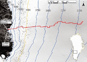
Fig. 1. Study site displaying model profile (red line) from the ice-sheet divide through Isunnguata Sermia to the western margin. Surface elevation contours (blue lines) are given in meters above sea level, and interpolated from Reference Bamber, Layberry and GogineniBamber and others (2001). The yellow contour at 1500ma.s.l. represents the approximate equilibrium-line altitude (ELA), according to Reference Van de WalVan de Wal and others (2008).
Methods
Field equations
Our model is built upon the continuum mechanical formulation of the laws of conservation of mass, momentum and energy for an incompressible fluid. These are, respectively,
where u is the velocity vector, σ the stress tensor, θ the temperature and Φ sources of heat generation in the ice. Physical constants cp
, k
i, ρ and g are defined in Table 1. Analysis is restricted to the x-z plane, or the vertical profile, making ![]() , where î and
, where î and ![]() are unit vectors in the x and z directions, respectively.
are unit vectors in the x and z directions, respectively.
Table 1. Parameters and physical constants used in the model

Conservation of momentum and mass
The constitutive relation for ice takes the form
where τij is the ij element of the deviatoric stress tensor, which is defined by τij = σij – pδij , with δij the Kronecker delta function. Isotropic pressure is defined as p = –⅓∑ i σii . є ij represents the corresponding element of the strain-rate tensor and η the viscosity. The strain-rate tensor is given by, and related to, velocity gradients as follows:
A non-Newtonian rheology is used for ice:
with ![]() , or the second invariant of the strain-rate tensor, and
, or the second invariant of the strain-rate tensor, and ![]() a regularization parameter introduced to avoid a singularity at zero strain rate. Glen’s flow law (Reference PatersonPaterson, 1994) gives n = 3. A(θ*
) is the flow law rate factor, given by Reference Paterson and BuddPaterson and Budd (1982):
a regularization parameter introduced to avoid a singularity at zero strain rate. Glen’s flow law (Reference PatersonPaterson, 1994) gives n = 3. A(θ*
) is the flow law rate factor, given by Reference Paterson and BuddPaterson and Budd (1982):
where θ* is the homologous temperature, defined by θ* = θ + bp, and R is the universal gas constant.
Under the assumption of steady state, the velocity of the ice is then determined from Stokes flow confined to the x-z plane,
and the conservation of mass, ∇u = 0.
Conservation of energy
Φ, the term in Equation (3) which represents internal heat generation, is computed as
Under the assumption of steady state and uniform thermal conductivity, the temperature of the ice is given by
Boundary conditions
Boundary conditions are applied to three distinct regions on the boundary of Isunnguata Sermia: (1) the surface; (2) the bed; and (3) a vertical boundary at the ice divide.
Conservation of momentum and mass boundary conditions
The surface of the glacier upholds the neutral or stress-free boundary condition:
where ![]() is the outward normal unit vector.
is the outward normal unit vector.
The bed of the glacier is subjected to a Weertman-style sliding law, where basal velocity and shear stress are related as
where β 2 is a positive scalar, spatially variable parameter representing the magnitude of frictional forces at the bed and τ b is given by
evaluated at the base of the glacier. We constrain the sliding velocity to be tangential to the bed, that is u
![]() =0.
=0.
The vertical boundary at the divide is subject to a symmetry boundary condition:
where ![]() is the unit vector tangent to the divide.
is the unit vector tangent to the divide.
Conservation of energy boundary conditions
The bed of the glacier is subject to an inward heat flux given by
where q g is the geothermal heat flux, q f is heating due to sliding friction and q l is latent heat associated with the melting of ice. q g is taken as 42 mWm–2, unless otherwise stated. Frictional heat is calculated as
Latent heat is given by
This heat interacts with the ice via the Neumann boundary condition
Note that the inclusion of the latent heat term serves as a temperature constraint on the ice by counteracting the inward flux from geothermal heat and frictional heat when the basal ice is at the pressure-melting point.
The surface temperature of the glacier is inferred from the dataset of Reference EttemaEttema and others (2009), and is imposed as a Dirichlet boundary condition. The vertical boundary at the divide is thermally insulated such that ![]() [−k
i
∇θ] = 0.
[−k
i
∇θ] = 0.
Model domain
The geometry for the model domain was derived from the surface elevation and thickness data of Reference Bamber, Layberry and GogineniBamber and others (2001). Since the model used here considers only a vertical profile, we selected a streamline from the surface velocity data presented by Reference Joughin, Smith, Howat, Scambos and MoonJoughin and others (2010). We employed cubic splines to interpolate the glacier geometry between data points, which were spaced at 5 km.
Due to the discrete nature of the original dataset, the profile surface contained numerous artifacts, manifested as irregularities in slope. In order to produce a more reasonable surface, we implemented a free-surface evolution scheme, and allowed the model geometry to relax for 50 years. The high driving stresses associated with the slope irregularities quickly diffused, yielding a surface free from the original artifacts, but still consistent with the data and model physics.
Numerical considerations
The model uses the finite-element method to solve the field equations subject to the boundary conditions. Lagrange quadratic elements are used (Reference HughesHughes, 2000), allowing second derivatives of the velocity to be computed accurately. The nonlinearity resulting from the viscosity (Equation (6)) is resolved using the modified Newton’s method iterative solver (Reference DeuflhardDeuflhard, 1974). The resulting linear systems were solved with UMFPACK (Reference DavisDavis, 2004). Model-specific parameters are summarized in Table 2. All numerical work was carried out in the Comsol Multiphysics modeling environment, a commercial package for finite-element analysis of general partial differential equations.
Table 2. Quantities of importance for model numerics
Modeling assumptions
Several assumptions were made in the development of this model, and results must be understood with these in mind. The assumptions are as follows:
The datasets used in the generation of the model domain geometry are sufficiently accurate, and the surface smoothing used to reduce artifacts does not introduce additional errors larger than those resulting from artifacts in surface geometry.
Stresses acting transverse to the dominant flow direction are small. This is necessary due to the effect that these stresses, and associated strains, have on the rheologic properties of the ice. Given the profile’s location at the center of the ice catchment, and the uniform width of the streaming feature, this assumption is likely to be valid.
The steady-state solution generated by the data-assimilation process is a reasonable representation of a long-term configuration for the model domain. This assumes that the modeled region of GrIS was not in a transient state when the data were collected.
A constant geothermal heat flux is an appropriate parameterization of the real phenomenon across the modeled domain. This is to say that, given the spatial scale under consideration, variability in geothermal heat flux is either of a sufficiently low resolution to be considered in an average sense, or of a sufficiently large scale that it is essentially constant.
Steady-state solutions which include the data-assimilation process are sufficient for probing the sensitivities of the system with respect to changes in the basal boundary. A more complete treatment would entail the evolution of the free surface to determine the ultimate outcome of the perturbation, but that is beyond the scope of this work.
Data assimilation and model initialization
When modeling ice dynamics, there are two issues that must be addressed before numerical experiments can be conducted. Firstly, fields which have not been directly measured but are significant in computing flow must be estimated. For instance, the internal distribution of temperatures is critical to ice dynamics, but is at best known at a few boreholes. We refer to this process as ‘model initialization’. Secondly, the initialized model should be in agreement with measurements that are available. We refer to this as ‘data assimilation’.
Our strategy in this paper is to use steady-state solutions to conservation equations to initialize the model, subject to the constraints introduced by the data-assimilation process. This is not a new idea: Reference MacAyealMacAyeal (1993) introduced control methods in the context of ice-sheet modeling. Here, we extend the concepts to solutions which incorporate the full flowline stress balance.
For data assimilation, we use the adjoint of the linear operator to compute derivatives of an objective function, and use these slopes to minimize the function. We have defined an objective function in terms of difference between the observed (u obs(x)) and modeled (u mod(x)) surface velocities,
which will be differentiated with respect to a parameter, p, that we vary in order to minimize the objective function. In this case the parameter is p = β(x)2, or the basal traction. Our introduction follows that of Reference StrangStrang (2007, p. 678–684).
‘Chain rule’ differentiation yields
where u is a solution vector containing both velocities and temperatures. The key to efficient calculation of the derivatives of the objective function is writing
or, recognizing that the objective function is linear in u. It is now possible to write the gradient as
where c T A– 1 is the result of solving the ‘adjoint’ linear system, A T λ = c for λ T = c T A– 1. Note that the original problem is assumed to be represented by the system of linear equations, Au = b. Hence, the gradient for each step of an optimization algorithm (we use quasi-Newton) requires a single extra linear solve, rather than a linear solve for each of the many parameters, p. This saving makes it possible to do large inverse problems, such as computing a basal traction for each point in the model domain (Fig. 2). Figure 3 corresponds to the initialized velocity and temperature field, or the steady-state solutions to the field equations that assimilate the data. This will provide the starting point for all numerical experiments. In some cases, such as determination of the sensitivity to q g, the entire assimilation/initialization process is repeated with different values.
Fig. 2. Top: modeled and observed velocity, as well as the portion of the modeled velocity accounted for by internal deformation. Middle: the β 2 field derived from the data-assimilation procedure. Bottom: the topography underlying the modeled ice profile.
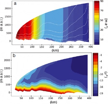
Fig. 3. (a) Velocity and (b) temperature fields produced by the data-assimilation process. White lines in (a) indicate flowlines within the velocity field.
Numerical Experiments
Sensitivity of the FMB to basal heat flow
In order to determine the sensitivity of the location of the FMB to different values of geothermal heat flux, we performed the data-assimilation procedure over a range of possible values. This experiment is motivated by the observation that basal sliding represents a significant portion of the total modeled surface velocity, and we wish to determine the geothermal heat flux required to produce a completely melted bed, in line with the assumption that the bed must be at the melting point for sliding to occur. We conducted model runs every 5 mWm–2 within the range 0–120mWm–2. Figure 4 shows the location of the FMB as a function of the prescribed geothermal heat flux. The FMB asymptotically approaches the divide as geothermal heat flux is increased, although the entire bed is not at the melting point under any of the parameter values considered, even for fluxes which seem unreasonably high. For comparison, previous authors have used a value of 42 mWm–2 (Reference PattynPattyn, 2003), and a structural similarity model by Reference Shapiro and RitzwollerShapiro and Ritzwoller (2004) indicates a mean geothermal heat flux of ~58mWm–2 along our flowline.
Fig. 4. Sensitivity of FMB location to variations in the geothermal heat flux.
Sensitivity of the FMB to sliding
Previous work suggests that seasonal changes in the glacial drainage system below the equilibrium-line altitude (ELA) can contribute to changes in basal traction, leading to changes in surface velocity (Reference Zwally, Abdalati, Herring, Larson, Saba and SteffenZwally and others, 2002; Reference Joughin, Das, King, Smith, Howat and MoonJoughin and others, 2008; Reference Van de WalVan de Wal and others, 2008; Reference Bartholomew, Nienow, Mair, Hubbard, King and SoleBartholomew and others, 2010). There is little agreement between these authors regarding the magnitude of proposed changes in surface velocity. Reference Joughin, Das, King, Smith, Howat and MoonJoughin and others (2008) suggest that terrestrially terminating glaciers in the region south of Jakobshavn Isbræ (of which Isunnguata Sermia is one) experience 25% increases in surface velocity as a result of surface meltwater lubricating the bed. Reference Bartholomew, Nienow, Mair, Hubbard, King and SoleBartholomew and others (2010) suggest speed-ups as great as 200%, and that a warming climate and associated surface lowering will expose greater portions of the bed to surface meltwater, increasing the fraction of the ice sheet exposed to summer speed-ups. Reference Van de WalVan de Wal and others (2008) acknowledge these seasonal variations, but present data showing an overall 10%decrease in surface velocities between 1990 and 2007. They also note that surface ablation and velocity show no correlation.
Regardless of the magnitude and sign of such changes in surface velocity, we sought to determine whether perturbations to the basal traction field, β 2, downstreamfrom the ELA, such as those which would be induced by increased surface meltwater production, would have an impact on the basal thermal regime, specifically the location of the frozen melted boundary. We tested this by inflicting constant multiplicative perturbations to β 2 downstream from the ELA, ranging between 50% and 200% of the value produced by the data-assimilation process. The location of the FMB was insensitive to all these perturbations. The reason for this is shown in Figure 5. Notable changes in the surface velocity field (>1ma–1) extend only 20 km, or ~10 ice thicknesses, upstream from the extent of the perturbation.
Fig. 5. Sensitivity of surface velocity to perturbations to the basal traction field, β 2. ELA is ~1500ma.s.l.We interpret the longitudinal coupling threshold (LCT) to be the location at which the difference between any two surface velocity profiles is ≤1ma–1.
Thus, the advection of heat away from the bed, the dominant mechanism accounting for heat flux at the bed, as shown in Figure 6, is unchanged 90 km upstream, at the location of the FMB. This short coupling distance within the velocity field is corroborated by other studies (Reference Price, Payne, Catania and NeumannPrice and others, 2008; Reference Bartholomew, Nienow, Mair, Hubbard, King and SoleBartholomew and others, 2010).
Fig. 6. Budget of (a) heat sources and (b) sinks along the profile basal boundary. Latent heat generation (not shown) is a negative nonzero term below the FMB, and accommodates excess heat generated from (a). Strain heat is a positive nonzero term, but negligible compared to frictional and geothermal heat sources.
Heat budget
In order to track the dominant factors which dictate the thermal regime at the bed, we calculated a heat budget of sources and sinks in terms of flux to the ice-sheet base. We performed this calculation for a model scenario with optimized β 2 and a geothermal heat flux of 42 mWm–2; results are displayed in Figure 6. Upstream of the FMB, frozen conditions are controlled by the advection of cold ice.
Near the divide this advection is predominantly vertically directed from the surface. Moving downstream, advection becomes bed-parallel, so the advective flux decreases to zero at the FMB as heat sources raise the ice temperature as it flows along the bed. Throughout the frozen zone, and some kilometers beyond the FMB, the primary source of heat along the bed is geothermal heat flux. We find that heat generation due to straining at the bed is a positive contributor, but negligible compared to geothermal and frictional sources. Downstream of the FMB, excess heat generation is accommodated by the consumption of latent heat associated with the phase transition from ice to water as basal melt occurs. Basal melting initiates at the FMB and steadily increases to a maximum of ~20mma–1 near the terminus.
Discussion
The sensitivity experiments described above indicate strongly different responses by the FMB to perturbations in geothermal heat flux and basal sliding. The direct response of the basal thermal regime to changes in geothermal heat flux is an expected result. However, the diminishing sensitivity of the FMB to increasingly higher heat fluxes is worth noting, and likely reflects the inability of the added heat to overcome cold advected from upstream.
In contrast, longitudinal coupling effects from sliding perturbations below the ELA do not propagate far enough up-glacier to influence the FMB. The location of the FMB is consequently insensitive to such perturbations. This interpretation hinges on the assumption that sliding perturbations apply only below the ELA, which is reasonable considering that the effect of increased surface melt input to the basal hydrologic system is not likely to propagate a significant distance upstream along the bed. We hypothesize that the limited distance over which longitudinal coupling occurs is a result of stress being dissipated at the basal boundary. It is important to note that sliding in our model is not limited to below the ELA. In fact, our optimization scheme produces a β 2 field with sliding above the FMB to the ice divide, albeit the upstream sliding is small relative to that occurring near the margin. Migration of melted conditions to the divide does not occur under very high values of geothermal heat flux, so the representation of sliding in our modeled frozen zone needs some explanation.
If the bed is in fact frozen we see several potential explanations for our modeled sliding. Firstly, sliding has been observed over a frozen bed consisting of a till layer (Reference Engelhardt and KambEngelhardt and Kamb, 1998), or hard bedrock (Reference Echelmeyer and WangEchelmeyer and Wang, 1987; Reference Cuffey, Conway, Hallet, Gades and RaymondCuffey and others, 1999). Additionally, substantial deformation has been observed within a frozen till layer, both within the body of the till itself (Reference Echelmeyer and WangEchelmeyer and Wang, 1987; Reference Engelhardt and KambEngelhardt and Kamb, 1998) and along discrete shear planes (Reference Echelmeyer and WangEchelmeyer and Wang, 1987). This mechanism may be taking place if such a layer exists beneath GrIS. Secondly, and perhaps more likely, our model could under-represent velocity from ice deformation, requiring our optimization scheme to over-represent sliding to maintain the observed surface velocity. Changes in flow due to variable impurity and water content and grain size of ice are not accounted for in our model; however, elsewhere in Greenland, a layer of soft pre-Holocene ice has been observed to enhance flows 1.7–3.5-fold (Reference PatersonPaterson, 1994; Reference Lüthi, Funk, Iken, Gogineni and TrufferLüthi and others, 2002). Alternatively, but in the same vein, the standard constitutive law we use could under-represent grain-scale ice deformation processes (Reference Goldsby and KohlstedtGoldsby and Kohlstedt, 2001). Finally, the velocity field itself could potentially depict a velocity field out of balance with the current ice-sheet geometry. We have no basis to eliminate any of these possibilities. However, if the magnitude of sliding over frozen bed computed here is not real, it is likely to be principally accounted for by spatial changes in geothermal heat flux, anisotropies within the ice, or a combination of the two.
An alternative scenario is therefore a partitioning of the observed surface velocity with enhanced ice deformation and reduced sliding velocity. Our heat budget along the basal boundary suggests the implementation of sliding has a significant influence on the location of the FMB by increasing the advection of cold ice along the bed. Under this alternative scenario, the associated drop in sliding velocity combined with additional interior heat generation from enhanced straining may modulate the cold contribution from advection, pushing the FMB further upstream. These processes would likely be countered by a decrease in frictional heating, which would force the FMB towards the margin. A model exploration of FMB migration from this interaction of heat sources is beyond the scope of this paper, but will be the focus of future work.
Conclusions
We have developed a thermomechanically coupled, two-dimensional flowline model and applied it to a terrestrially terminating glacier profile located in western Greenland. We extracted geometric information for the model domain from a dataset presented by Reference Bamber, Layberry and GogineniBamber and others (2001), which we believe represents the best data available at present for the Greenland ice sheet. We used adjoint methods to optimize the basal traction field, such that modeled surface velocities matched observed values (Reference Joughin, Smith, Howat, Scambos and MoonJoughin and others, 2010) to within 1 ma–1.
With an optimized model in hand, we conducted experiments in order to determine the sensitivity of the FMB to perturbations in the basal heat flux and basal traction downstream of the ELA. We found that the FMB migrates easily under different assumptions about geothermal heat flux. At values close to 0mWm–2, the FMB moves very close to the terminus, but part of the bed remains unfrozen due to frictional heating from sliding. At high values, the FMB asymptotically approaches the ice divide. We found that for reasonable perturbations to basal traction downstream from the ELA, such as might be expected from an increase in surface meltwater production and associated bed lubrication, the FMB was insensitive. This is a result of the short length scale over which longitudinal stress coupling in the ice operates (~10 ice thicknesses). The FMB is significantly further upstream from the ELA than the perturbations to the velocity field extend, so advective heat fluxes are unchanged. Our model predicts that, under most assumptions about geothermal heat flux, sliding occurs over a frozen bed. We see two possible explanations for this: (1) that this sliding is real, and follows one of the mechanisms proposed by Reference Echelmeyer and WangEchelmeyer and Wang (1987), Reference Engelhardt and KambEngelhardt and Kamb (1998) or Reference Cuffey, Conway, Hallet, Gades and RaymondCuffey and others (1999); (2) anisotropies or variability in hardness within the ice result in a preferential flow direction and increased deformation. Additional work is needed to quantify the sensitivity of the basal thermal regime to the second of these factors.
Acknowledgements
Funding for this work was provided by the Greenland Analogue Project (GAP), a collaborative project funded by the nuclear waste management organizations in Sweden (Svensk Krnbrnslehantering AB), Finland (Posiva Oy) and Canada (NWMO). It was also funded by grants from the US National Science Foundation: NSF-CMG-0934404 (J.V.J.) and NSF-OPP-0909495 (J.T.H.).


