


1. Introduction
Pure powder avalanches are very rare in the Alps, while dense or mixed avalanches comprising a dense core covered by a powder layer are more frequent. In February 1999, a mixed avalanche overflowed the defence system built up in 1991 at the Taconnaz avalanche path, Haute-Savoie, France, showing the limits of the defence structure set up in 1991, especially against rapid and dry avalanches (see Fig. 1). The local municipalities decided to improve the system. Both dense and powder avalanches have to be considered in the defence-structure design: the defence structure must retain dense avalanches up to the centennial event and reduce the pressure developed by the powder part. Accordingly, Cemagref was asked by the municipalities to predetermine the dense-avalanche hazard at the entry to the defence-structure system; to design the best combination of defence structures able to spread the flow, dissipate the energy and retain the dense reference avalanche; and to analyse the residual risk due to the powder part of the avalanche.

Fig. 1. Photograph of the February 1999 avalanche deposit at Taconnaz, showing the lateral and frontal overflows.
In section 2 of this paper, the Taconnaz avalanche site is presented. Its morphology and its starting zones are analysed, and the available historical data related to meteorology and avalanches are presented, along with a statistical analysis of snow precipitation. In section 3, a back analysis of the historical avalanche data is undertaken using a numerical model. This allows the flow descriptors at the entry to the runout zone to be determined. In section 4, a statistical analysis is developed and applied to predetermine the volume and the Froude number. A bivaried approach is then developed and applied to predetermine centennial events according to these variables. In section 5, we use a small-scale laboratory model to optimize the shape, dimensions, location and numbers of the dissipative structures at the beginning of the runout zone. In section 6, we use an existing analytical approach, calibrated using the February 1999 avalanche data, to determine the height of the terminal catching dam devoted to stopping the dense avalanche. We also validate the whole system using a small-scale model and a two-dimensional (2-D) numerical model. In section 7, we study the effect of the catching dam on the powder phase in order to analyse the residual hazard due to the powder part of the Taconnaz avalanche. In section 8, we highlight the main technical and scientific outcomes of this project.
2. The Taconnaz Avalanche Path
2.1. Morphology
The Taconnaz avalanche path is located in the Arves valley close to Mont Blanc in France. During the last century several large dense and mixed avalanches occurred on this path, on several occasions reaching the inhabited areas. The starting-zone surface, the length and the drop at changes in the level of this path are exceptional (see Fig. 2). The immensity of the starting zone is the chief characteristic of the path. We identified at least three major starting zones. Between 3300 and 4000 m a.s.l., a vast glacial area with a surface of 2.0 × 10⁶m2, of highly irregular morphology, of mean slope 30° and oriented (northwest/northeast) leeward of the dominant winds represents a privileged snow deposition area. Its upstream and downstream ends comprise long lines of seracs, with a significant slope rupture representing a preferential release line. The potential release volume from this starting zone alone exceeds 4.0 × 10⁶m3. A second starting zone is located downstream between 2800 and 3300 m a.s.l. with a surface of 0.8 × 10⁶ m2. These two zones feed a 400 m wide, 1800 m long flow area with a mean slope of 31°. In this area, an additional significant snow volume can be eroded by the avalanche. Downstream on the right side, a lateral starting zone with slope 25°, length 800 m and width 300 m is located between 2000 and 2600 m a.s.l. Downstream of 2150 m a.s.l., the path is prolongated by a long flow zone with a 30° slope, 300 m wide and 900 m long. At 1700 m a.s.l. the avalanche meets a glacial moraine approximately 80 m high. High-speed powder avalanches can overrun it, but most avalanches deviated to the left of it. After the moraine, the avalanche enters its runout zone with a 13° slope (see Fig. 1). The historical records show that the difference between the maximum and minimum runout distances is >1000m. The Taconnaz path is 7 km long, has a mean slope of 25° and a mean width of 300–400 m.
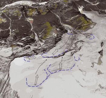
Fig. 2. The Taconnaz watershed morphology where the main starting zone areas are drawn (from www.geoportail.fr).
2.2. Centennial 3day cumulative snow precipitation
The analysis of existing daily meteorological data recorded at Chamonix (1042m a.s.l.), Vallorcine (1300ma.s.l.) and Les Houches (1008 ma.s.l.) allowed the centennial cumulative precipitation over 3days in each location to be predetermined. Assuming a snow density of around 130 kg m−3, the snow depths corresponding to the centennial precipitation are reported in Table 1 .
Table 1. Centennial 3 day cumulative precipitations (m) (source Météo France). Local adjustment of GEV model. Durations of the records at Vallorcine, Chamonix and Les Houches are respectively 40, 77 and 32 years
According to Reference Durand, Laternser, Giraud, Etchevers, Lesaffre and MérindolDurand and others (2009), at the Mont Blanc mountain scale the mean annual cumulative precipitation vertical gradient is 3.81 mm m−1 for a mean annual cumulative precipitation of 8.85 m. If we apply this vertical gradient to Les Houches (1008ma.s.l.) data, the 3day cumulative precipitation at the starting zone of the Taconnaz avalanche path (3300 ma.s.l.) is 1.6–2.3 m, with a mean value of 2 m.
2.3. Historical data
A permanent avalanche survey (Enquête Permanente sur les Avalanches (EPA)) has been organized by the French Forest Service since the beginning of the 20th century. The collected data contain qualitative and quantitative information. Among the quantitative data, the release and runout altitudes are systematically recorded (see Fig. 3 for the Taconnaz data). The mean length, mean width and mean thickness of the deposits in the runout zone have also been recorded for 49 events. We used these dimensions to estimate the volume of the deposit for each documented event (see Fig. 4).
Fig. 3. Topographical profile and historical data related to starting and runout altitudes.
Fig. 4. Historical runout distances and altitudes versus deposited volumes.
EPA suffers, like all avalanche databases, from different quality problems. For safety reasons, the rangers in charge of observation do not directly measure release and runout altitudes as well as deposit volumes, but estimate them from a distant observation point, generally using binoculars. This makes high observation errors unavoidable. For example, the uncertainty level around the stored runout altitudes was at least 50 m at the beginning of the record because of the imperfection of topographical maps at that time, but it has dropped to <10m today due to the availability of better maps and global positioning systems. For release altitudes, observation error is much higher, presumably at least 100 m. Finally, for deposit dimensions, the uncertainty level is extremely hard to quantify. It is presumably relatively small for deposit mean length and width, but is at least 20–30% for snow depths. Consequently, the recorded deposit volumes must be considered much more as rough estimates of the avalanche magnitude than as precise measurements of the mass involved.
3. Back Analysis of Dense Avalanches Using a 2-D Numerical Model
Dense-flow avalanches (including the dense cores of mixed avalanches) are considered in this section. All historical data were back-analysed using an avalanche-dynamics numerical model based on the following assumptions (see Reference Naaim, Naaim-Bouvet, Faug and BouchetNaaim and others, 2004): (1) the snow is considered as a quasi-incompressible fluid; (2) the flow is considered as shallow and its dynamics is controlled by a basal thin and strongly sheared layer comprising snow particles, whereas the core comprises grains and large aggregates (inducing a much weaker shear rate); (3) the stress distribution is considered to be quasi-isotropic; and (4) the effective friction at the base of the flow is considered to be represented by the Voellmy model (Reference VoellmyVoellmy, 1955). The shallow-model equations are:
where h is the flow depth, u and v are the velocity vector components in the x (east-west) and y (south-north) directions respectively, z s is the terrain altitude, a is the slope angle, Cx and Cy are the terrain curvatures and <p is erosion or deposition flux as defined by Reference Naaim, Faug and Naaim-BouvetNaaim and others (2003). These equations are solved using a 2-D finite-volume scheme based on a simplified Riemann solver (Reference Naaim, Naaim-Bouvet, Faug and BouchetNaaim and others, 2004). The model takes into account the terrain topography through the local slopes and curvatures on a refined grid (5 m). The initial snow distribution is introduced as a 2-D grid. In order to back-analyse each avalanche, the initial conditions were defined as follows. The starting zone is defined according to the starting-point altitude. For the initial volume, we assumed equality between erosion and deposition along the path and fixed the initial volume equal to the deposited volume. Afterwards, we fixed £to 1500 m s−2 because the path is open and the main flow zone is covered by Glacier de Taconnaz. We iterated model calculations, varying the friction coefficient μ 0 until the avalanche runout altitude was equal to the observed runout altitude. The obtained friction coefficients μ0 are plotted in Figure 5 according to the runout altitudes. They range between 0.15 and 0.35. Figure 5 shows a significant correlation between the runout altitude and the friction coefficient μ0. We also plotted the latter according to the volume, in order to show the weak correlation between the volume and the friction coefficient (see Fig. 6). The correlation with the corresponding volumes is <0.3, so we consider the two variables as quasi-independent in section 4.
Fig. 5. Back analysis of historical data using numerical simulations: the obtained effective friction coefficient μ0 versus the runout altitude.
Fig. 6. Back analysis of historical data using numerical simulations: the deposit volume (m3) versus the effective friction coefficient μ 0.
For each avalanche, the height and velocity variations according to time of entry into the runout zone (1240m a.s.l.) were recorded and analysed. The Froude number, F, defined as the square root of the ratio between the kinetic and the potential energies, and corresponding to the maximum discharge, was determined for each avalanche. The obtained Froude numbers are plotted in Figure 7. They are highly correlated with the friction coefficient μ0 (friction coefficient of the avalanche close to its rest).
Fig. 7. Back analysis of historical data using numerical simulations: the Froude number versus the effective friction coefficient μ 0.
4. Statistical Analysis
4.1. Predetermination of avalanche volume and Froude number
The predetermination of high return periods requires a probabilistic model (Reference Eckert, Parent, Naaim and RichardEckert and others, 2008) and requires considering the data as realizations. This model is assumed to belong to a family of probability laws characterized by a set of parameters to be estimated using a statistical procedure. ‘Peak over threshold’ (POT) modelling considers only data above a certain threshold. The number of used data is reduced, but the determination of rare quantiles is more precise because calibration is primarily performed on the highest values. Moreover, the problem of model choice is considerably simplified by the convergence of the exceedances of any so-called max-stable process towards well-known limit laws (Reference PickandsPickands, 1975). In fact, under the hypothesis that the threshold m is high enough, the set of k independent exceedances in T years behaves like a Poisson process whose probability distribution p is indexed by a single parameter 77 (Equation (3)). The exceedances y are distributed according to a generalized Pareto law whose cumulative distribution F indexed by the parameters (<5,/3) is given in Equation (4). A crucial role is played by the shape parameter β defining the attraction domain, i.e. the increment of the quantile with return period. The main practical problem for the implementation of POT modelling is the choice of the threshold: it must be high enough to ensure the convergence of the asymptotic model, but low enough to retain a satisfactory number of data. A good empirical way to determine m is to represent the arithmetic mean of the exceedances as a function of the threshold, and select the threshold that corresponds to the beginning of the linear graph (Reference ColesColes, 2001).
For the volumes, the retained threshold is 0.25 Mm3, keeping 20 data corresponding to the distribution tail. The parameters (η, β, δ) of the POT model were inferred under the Bayesian paradigm with a non-informative prior (Reference Parent and BernierParent and Bernier, 2003). We systematically tested the three models (β > 0, β = 0 and β < 0) and retained the model (β > 0) because it maximizes the Bayes factor (Reference Kass and RafteryKass and Raftery, 1995). The matching between the data and the model, though not perfect, is satisfactory as shown in Figure 8. The fitting is very good for values between 0.5 × 10⁶ and 1.5 × 10⁶m3. On the other hand, the exceptional volume (4.3 Mm3) of 1950 is difficult to take into account. For the Froude number, a limited sample of 20 data exceeding 1.82 was retained for the statistical analysis. The Bayes factor clearly selected the Weibull domain of attraction corresponding to a positive value of β. The Froude number distribution is bounded by a Froude number limit of 6.92. The matching between the data and the model is satisfactory (see Fig. 9). Equations (3) and (4) are inversible, allowing analytical expression of the quantiles corresponding to any annual non-exceedance probability, i.e. any return period. Centennial values are 3.58 for the Froude number and 1.6 Mm3 for the volume.
Fig. 8. Matching between the volume data and the predictive law.
Fig. 9. Matching between the Froude number data and the estimated POT model.
4.2. Bivaried analysis
Results obtained by marginal analyses of volumes and Froude numbers remain to be considered to define the reference events. The statistical treatment of the distribution of extreme values of a bivariate process is a very complex issue and is still under investigation. The main difficulty is the existence of an infinite number of limit models (Reference Coles, Heffernan and TawnColes and others, 1999). In our case, the problem is greatly facilitated because the two variables V and F are assumed independent. The non-exceedance probability of a doublet of values defining a return period is then simply the product of the corresponding marginal probabilities of exceedance. Thus there is an analytical relationship f between V and F for a given return period T given by Equation (5), where subscript 1 refers to the volume and subscript 2 to the Froude number. This relationship defines an envelope curve of the couples (F, V) corresponding to a given return period T. It induces that, for a given return period, increasing V corresponds to a decrease in F, and vice versa. Figure 10 presents the envelope curves for three classical return periods. Given the selected attraction domains, there is a limit Froude number but no maximal volume. For a given return period, marginal values are also limit values. For example, for a return period of 100 years, the marginal centennial volume is the smallest possible, whereas slightly higher volumes correspond to very high Froude numbers, and much higher volumes to more reasonable Froude numbers. Note also that the observed data correspond from this bivariate point of view to relatively small return periods. The 1950 event, for example, had an exceptional volume, but a relatively low Froude number, so its return period is only around 20 years. We retained several doublets (F, V) corresponding to the centennial events.
Fig. 10. Envelope curves for different return periods versus data.
In the following, and as an example, we analyse the design of the new defence structure considering only one centennial doublet (F=4.29, V= 1.6 × 10⁶ m3), keeping in mind that we considered several other doublets in the technical study.
5. Physical Modelling and Mound Design
In the literature, several studies have been devoted to mound effects on dense granular avalanches (Reference Hákonardόttir, Hogg, Jόhannesson and TόmassonHákonardόttir and others, 2003; Reference Jόhannesson and HákonardόttirJόhannesson and Hákonardόttir, 2003). They showed that the runout shortening was proportional to the mound height relative to the incoming flow height. According to numerical simulations of the historical events, the flow height corresponding to the maximum discharge at the entry to the runout zone is around 10 m. According to Reference Hákonardόttir, Hogg, Jόhannesson and TόmassonHákonardόttir and others (2003), the optimal height of the mounds is around 1.5 times the incoming flow height. We could not extend the height of the mounds to meet this rule of thumb, because the construction of such mounds would have involved several inconveniences in terms of landscape and costs. We limited the height of the mounds to 7.5 m, and studied different lengths and combinations of mounds. To this end, we developed a specific small-scale physical model to study and optimize the mounds in terms of energy dissipation and flow spreading. To compare the effectiveness of various configurations of the protection device, we relied heavily on small-scale physical modelling. The relevance of this technique has been widely demonstrated within the framework of the achieved European projects CADZIE (Catastrophic Avalanches Defence structures and Zoning in Europe) and SATSIE (Avalanche Studies and Model Validation in Europe).
5.1. Principle of the physical modelling
A simplified small-scale model (scale 1:500) of the runout zone was built as shown in Figure 11. The model is fed with granular flows using an inclined channel with an adjustable slope, equipped at its top with a reservoir where the avalanche volume is initially stored. A dimensionless analysis of the depth-averaged equations highlights three similarity criteria: (1) the geometry ratio, (2) the Froude number F 2 = U2/gH and (3) the difference between the slope angle and the basal friction angle (tanθ – μ). The mean slope of the reduced model is equal to the mean slope of the runout zone of the real path (13°). The adjustable slope of the channel allows the desired velocity and Froude number to be fixed at the entry to the runout zone. The second similarity criterion is then fulfilled. The granular material used was chosen after several calibration tests. We added different proportions of PVC beads of diameter 0.1 mm to glass beads of diameter 1 mm. We measured the runout distance obtained for different proportions and chose the proportion corresponding to the maximum observed historical runout. The chosen bi-disperse material had final proportions of 10% PVC beads and 90% glass beads. Close to the stopping phase, the experimental value of (tan θ – μ) is then similar to the observed data. We considered the third similarity criterion fulfilled even if this is strictly correct only when the avalanche comes to rest. One major problem we had to confront during the experiments was the uncertainty evaluation. Because the initial conditions are never identical and the system is somewhat chaotic, the obtained runout distances for two tests with the same initial volume and the same granular material could vary. To take these variations into account, we systematically realized five tests in the same conditions and calculated the mean value and standard deviation. The latter was around 4 × 10⁻² m (20 m). The comparison between the various configurations was done using the mean values and the standard deviations.
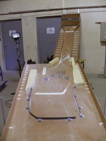
Fig. 11. Photograph of the small-scale physical model of the runout zone, inclined at 138, fed with granular flows from a channel of adjustable slope, and equipped with a reservoir at the top to store material before the granular avalanche release.
5.2. Mound-design results
The purpose of the mounds is to dissipate the energy and spread out the flow. We considered several rows. As a first step, we studied the shape of the mounds and their location in the first row using the scale model where the mounds were set up alone. The width of the dense part of the avalanche at the beginning of the runout zone is 50–100 m. In terms of runout shortening and spreading, the best result was obtained with two large mounds (height 7.5 m), with an open section between them of 30 m. The central part of the upstream face of each mound is a 7m wide rectangle normal to the slope and to the flow direction. This surface is prolongated at each side by a triangular surface forming an angle of 30° with the incoming flow direction. The total mound width, normal to the incoming flow, is 14 m. For the second row of mounds, the shape was kept the same. We set up a mound downstream, and in quincunx with the two mounds of the first row. We varied the downstream distance and measured the runout shortening. A distance of 80 m downstream face to face increases the total runout shortening of approximately 10%. Furthermore, the centre of lateral jets produced by the mounds in the first row reaches 60 m. We added two other large mounds to the second row, one on the left and one on the right, the central surface being located at the lateral jet impact. These two mounds produced additional runout shortenings of up to about 15% and increased the flow spreading on both sides. In order to increase the spread of the flow (and increase the flow surface) towards the right-hand side, we added one large mound 80 m downstream of the second row. This is located at the impact point of the lateral jet produced by the mound on the extreme right of the second row. The flow is then spread out so it reaches the mountains on the right and left of the runout zone. All the mounds that were finally designed are shown in Figure 12.
Fig. 12. (a) Top view of a large retarding mound (the thick lines indicate that the upstream face is protected by a grouted rock riprap revetment). (b) View of the upstream face of a large retarding mound normal to the incoming avalanche flow. (c) Spreading effect induced by the three rows of mounds, shown by laboratory tests and depicted here by the dashed-line white arrow; the plain arrow shows the main direction of the incoming avalanche flow.
6. Retention-Dam Design and Validation of the Whole System
6.1. Retention-dam design using an analytical method
In order to design the height of the terminal catching dam, we first used the classical empirical formula proposed by Reference SalmSalm (1982) and widely used in engineering studies. It is based on energy conservation. The sum of the kinetic and potential energies (ρgh+1/2ρV 2) of the incoming flow is transformed into potential energy of the avalanche after stopping (ρgR, where R is the run-up) and into energy dissipated during the interaction between the avalanche and the dam (1/2γσv 2). This leads to:
In order to calibrate the dissipation coefficient γ, we used the run-up of the February 1999 avalanche. The observed deposit left by the 1999 avalanche was measured over a large area. The average height above the dam (which is 14 m high) was 3 m. The observed run-up was then at least 17 m. The estimated deposited volume was 0.8 × 10⁶ m3. For a channelized flow, Reference Chambon and NaaimChambon and Naaim (2009) obtained a simple linear relationship between the flow height at a given location and the avalanche volume. This relationship can be extrapolated to 3-D avalanches if one assumes that lateral spreading is proportional to the avalanche height. At a given location, the 3-D flow height of an avalanche flowing over an open slope is then proportional to the square root of the volume. Moreover, according to the Voellmy friction law, the Froude number depends mainly on the slope and the friction parameters. At a given location we can then simply relate the run-up to the volume as follows:
The application of Equation (7) leads to a run-up of at least 24 m for an avalanche volume of 1.6 × 10⁶ m3 with a Froude number equal to that of the February 1999 avalanche.
6.2. Validation of the whole system using physical and numerical simulations
In order to test the whole system, we first used the numerical model based on Equations (1) and (2). This model had already been used successfully to back-analyse the 1999 event (Reference Naaim, Faug and Naaim-BouvetNaaim and others, 2003). The runout zone was modelled by a refined grid of 1 m space step. The topography of the runout zone was modified to take into account the new defence structures. Each cell is afterwards represented by its new slopes and curvatures. The friction parameters are those of the reference event. Even when, during the interaction between the flow and a given defence structure, the numerical model accounts only for the energy loss produced by the deposition, the shocks and the curvature, very good agreement is found when comparing the results of the small-scale model to those of the numerical model. The hydrograph imposed as the boundary condition at the top of the runout zone was varied from a decennial to a centennial event, the latter corresponding to the reference event. In parallel, we used the reduced physical model to simulate the same tests. Both the physical and the numerical models showed an overflow downstream of the terminal dam for the centennial event, especially on the left-hand side. This is mainly due to the left-side morphology. Indeed by moving the current right-side lateral dam, the flow could extend its width and reduce its height on the right-hand side, whereas the mountain on the left-hand side is too close and avoids the benefit from extra lateral spreading. The flow is rapidly reoriented towards the central part of the device. To overcome this problem, we supplemented the system of mounds by adding, in the middle of the runout zone, a transversal dam 120m long and 7m high (see Fig. 12). This modification was successfully tested using the numerical and physical modelling. The obtained deposits are shown in Figures 13 and 14 respectively. Using the numerical and physical models, we also varied the volume of the avalanche from 0.5 × 10⁶ m3 to 2.0 × 10⁶ m3 and we compare the obtained run-up at the level of the terminal dam to the results predicted by the simple analytical Equation (7) in Figure 15. The analytical predictions are close to the results obtained using the numerical and the experimental data. Finally we analysed the efficiency of the defence system against two successive decennial events occurring in the same year. For the first event we used two alternatives: high volume with low Froude number, and high Froude number with low volume. In the first case, the deposit obtained fills the mounds, whereas in the second, the deposit reaches the terminal dam. The deposit left by each of these events is used to modify the digital terrain model. Over this new terrain model, we analysed the flow of a new decennial event. The deposit contained the second event in both cases.

Fig. 13. Final deposits given by experimental simulations.

Fig. 14. Final deposits given by numerical simulations.
Fig. 15. Run-up (m) at the terminal catching dam versus the avalanche volume (m3): comparison between analytical, experimental and numerical results.
7. Effects of Powder Avalanches
The powder avalanche study was undertaken using physical and numerical modelling. In a large water tank, the flow of salt-water solution supplemented with particles of kaolin was used to simulate the inertial phase of the flow of a powder avalanche. A computational fluid dynamics (CFD) numerical model similar to that of Reference Sampl, Naaim-Bouvet and NaaimSampl and others (2004) was first used to simulate the same physical experiments in order to be calibrated. It was then used with a realistic density ratio to analyse the effect of the dam on the avalanche pressure downstream of the terminal dam.
7.1. Physical experiments
The Taconnaz site is a huge avalanche path, and a 100 m powder avalanche height is likely to occur. However, we limited the reference height to 50m in order to perform accurate numerical simulations with obstacles of 14 and 28 m. This reduction of the avalanche height will not induce a significant distortion because, according to Reference Sampl, Naaim-Bouvet and NaaimSampl and others (2004), the variation of the dissipation coefficient for a flow of 50 m over obstacles of 14 and 28 m is similar to the variation of the dissipation coefficient of a flow of 100 m over obstacles of 14 and 28 m. A series of experiments was then undertaken in the case of an avalanche 50 m high with a front velocity of 30 ms−1 over a 2-D small-scale model of 10° slope, and two dams of 14 and 28m were tested. The results obtained are displayed in Figure 16. If we compare the front velocity, we can see clearly that the 28 m dam does not contain the powder avalanche, but the front velocity of the avalanche is greatly reduced compared to the velocity of the avalanche with the 14m dam.
Fig. 16. Ratio of the front velocity of the avalanche with the dam and the front velocity of the avalanche without the dam versus the downstream distance.
7.2. Numerical simulations
A series of numerical experiments was also undertaken to study the case of a powder avalanche 50 m high with a front velocity of 30 m s−1 and mean density ratios of 1.2 and 4 over a 2-D small-scale model of 10° slope. Two dams of 14 and 25m were taken into account (see Fig. 17). The first series of tests with a density ratio of 1.2 and the 14m dam were dedicated to demonstrating the validity of the numerical simulations compared to the experimental data. The second series of experiments with a density ratio of 4 took into account the effect of density, which reduces the ambient fluid incorporation as shown by Reference Sampl, Naaim-Bouvet and NaaimSampl and others (2004). The simulations showed that the dam height increase leads to a reduction of pressure everywhere in the dam downstream area. In the inhabited area, the pressure is reduced by up to 50% by the 25 m dam compared to the 14m dam, representing a significant gain in terms of risk reduction.
Fig. 17. Ratio of the pressure obtained by a dam of 25 m and a dam of 14 m versus the downstream distance (pressures are measured at 10m from the ground).
8. Discussion and Conclusion
The main interest of this paper is to show how recent scientific developments could be used to solve an avalanche engineering problem related to the design of a defence structure system. This study concerns the Taconnaz avalanche-path defence system. We used recent advances in analytical and statistical methods, as well as physical and numerical modelling of dense and powder avalanches.
Recent statistical developments combining historical data and numerical propagation models were successfully used to predetermine bivariate reference events. We considered the avalanche volume and the Froude number as two pertinent descriptors for studying avalanche interaction with obstacles. Future research should tackle the issue of possible dependence between the flow descriptors. It is important to note that we could not have undertaken such an in-depth study had the historical data been sparse, as in the case of the majority of avalanche paths. Transferring existing knowledge from one path to another is therefore another future challenge.
The physical modelling widely used in recent scientific developments was used here as an engineering tool. Using a special procedure, we showed how an adequate choice of granular material can allow the similarity criteria to be fulfilled. A bi-disperse granular material with fine PVC particles and larger glass beads was used. A weak proportion of fine particles was shown to be relevant for simulating the observed deposits, not only in terms of maximum runout but also in terms of general features of the avalanche deposits (mass spatial distribution, fingering and tongues). From our point of view, investigating polydisperse granular materials should bring future progress in modelling dry snow avalanches with small-scale physical models.
We also showed how numerical modelling based on a shallow-flow assumption can be applied to design a defence structure including complex topography. The numerical modelling of dense avalanches was successfully tested on experimental data and was used as an operational tool to design a complex avalanche protection system. A crucial point here is the erosion and deposition model included in the model, which allows better simulation of the avalanche in the runout zone (transition towards stopping) and the effects of obstacles. This model, validated only on granular material flows over rough inclines, still needs to be improved and validated on available data with full-scale observations.
Finally we applied a combination of gravity-current simulations (low density ratio) in a water tank and CFD numerical modelling (realistic density ratio). This provides an operational solution for determining the pressure reduction downstream of a defence structure and also allows access to the residual risk.


