


Introduction
Avalanche defence structures can minimize damage from snow avalanches or even prevent avalanche release. Although model experiments on various defence structures have been conducted previously (Reference Tai, Wang, Gray, Hutter, Hutter, Wang and Beer Tai and others, 1999), how to estimate the effectiveness of such structures has yet to be established. At present, the design of avalanche defence structures is mainly based on empirical laws. However, from the perspective of both safety and economics, a stronger and more rational physical basis is desirable. In addition, direct observations and measurements of avalanches are relatively scarce (e.g. Reference GauerGauer and others, 2007; Reference Sovilla, Schaer and RammerSovilla and others, 2008), and a reliable numerical model that can be used for full-scale avalanche analysis is required.
There are several available models that can predict the velocity and run-out distance of avalanches (for a short review see Reference Oda, Moriguchi, Kamiishi, Yashima, Sawada and SatoOda and others, 2011). However, these tools use depth-averaged approaches that do not allow the vertical velocity and pressure distribution to be calculated.
In this paper, we present a new approach that considers a snow avalanche as non-Newtonian fluid and also includes erosion and deposition processes. With this model, a fully three-dimensional simulation, which also reproduces the avalanche surface movement, becomes possible.
MPS Method
The moving particle semi-implicit (MPS) method was first proposed by Koshizuka (1996) and does not yet seem to be widely known. Here we briefly explain the basics of the MPS method.
As the name suggests, the MPS method is a computational technique that uses a particle (Lagrangian) approach with a semi-implicit algorithm. However, it does not perform calculations on every distinct particle of a particle body. Instead, the differential equations describing the behavior of a continuous body are discretized using the model of interacting fictitious particles.
In this study, the continuity equation
and the momentum conservation equation
for incompressible fluid are the base equations for avalanche simulations, where ρ is the density of particles, u is velocity, p is pressure, ν is the kinematic viscosity coefficient and g is the acceleration due to gravity. The velocity term is not included in Eqn (1) because of the formal property of the Lagrangian approach.
The model of interaction between particles is based on the weight function
According to this weight function, particles interact if the distance r between them is less than the r e parameter. At farther distances the interaction is assumed to be zero. At nearly zero distances the weight function approaches infinity, preventing particles from being too close to each other.
To express gradient and Laplacian operators of some physical parameter ϕ of a particle k through the weight function, the following equations were derived:
Here r is the position vector of a particle, d is the dimension (usually 3) and n 0 is the initial number density that can be known from the initial particle distribution. The value of the normalizing coefficient ⋋ can be found by
The number density can also be expressed through the weight function:
It should be noted that although each particle is treated locally, the same calculation is applied to all particles covering the whole area. Such local interactions are considered to be sufficient to recover the global equations (1) and (2).
To solve the momentum-conservation and continuity equations numerically, we use the so-called semi-implicit algorithm, where the pressure gradient term is implicit (m+1 index) but the viscosity and gravity terms are explicit (m index).
The calculation algorithm consists of two main stages: explicit and implicit. The details of each stage are described below.
Suppose that position vector r m , velocity u m and pressure pm of a particle for time-step m are known. The corresponding values for the next time-step, m+1, are subjects to be found. In the first step, find the temporary values of position and velocity of the particle using only the explicit terms of Eqn (9),
where the viscosity Laplacian term can be calculated by Eqn (5).
From these temporary values we obtain a new number density, n *, that differs from the initial value n 0. The point of the next stage is to find correction values of the velocity u' and the number density n' using the still unused implicit term (pressure gradient) in Eqn (9) and the difference between the temporary and the initial values of the number density.
The velocity correction term arises from the pressure gradient.
Next we use the following mass conservation law to exclude the difference in the density value:
Because density is proportional to the number of particles in the MPS method, ρ can be replaced by n, and after discretizing we obtain
Note that the correction values n' and u' are used here instead of n and u. Combining this equation with Eqn (15) we obtain the following discrete Poisson equation:
Applying Eqn (5) we obtain a system of linear equations from which the pressure pk +1 can be found for each particle.
Finally we should mention how free surface and wall conditions are set in the MPS method. Because there are no particles outside the avalanche body, the free surface can be determined by a decreased value of the number density (Fig. 1).
Fig. 1. Particles that can be determined as free surface. r e is the influence radius.
where β can be 0.95 or 0.97 according to Reference Koshizuka and OkaKoshizuka and others (1996).
By contrast, the wall is considered as two types of particle layers with fixed coordinates. The outer layer consists of particles that are both unmovable and non-calculable, while the particles of the inner layer are subjected to pressure calculation (Fig. 2). Because the influence radius may overlap several rows of particles, the layer of particles should be thick enough, i.e. consist of several rows of particles, otherwise it may mistakenly be considered as free surface. Sometimes the wall particles should be placed closer to each other to prevent particle leakage through the wall (Fig. 3).
Fig. 2. Wall particles layout.
Fig. 3. Layout preventing particle leakage through the wall.
Bingham and Dilatant Fluid Model
The Bingham fluid model describes materials that behave as a rigid body at low stresses but flow as a viscous fluid at high stress. The relation between shear stress and shear rate is
Here 0 is the critical value of the stress, below which there is no shear, and is the dynamic viscosity. A biviscous Bingham model was first adopted to describe avalanches by Reference Dent and LangDent and Lang (1983).
We propose that the system behaves as a Bingham fluid only when the shear rates are lower than some limit value which was determined empirically. At shear rates higher than it switches to dilatant fluid behavior that describes fluids with increasing viscosity.
The dependence of shear stress on shear rate for the combined Bingham–dilatant fluid model is shown in Figure 4.
Fig. 4. The constitutive law for combined Bingham–dilatant fluid model.
After rewriting Eqns (20) and (21) in terms of the dynamic viscosity η, we obtain the following final constitutive equation that was used in the simulations.
where η' is the Newton fluid equivalent of the dynamic viscosity and m is the stress growth coefficient. The last term of the first equation is introduced to approximate the Bingham fluid behavior at very low (near-zero) shear rates.
A similar rheology was also proposed in the Herschel– Bulkley model (Reference Kern, Tiefenbacher and McElwaineKern and others, 2004) which is appropriate at low shear rates and based on a two-dimensional depth-average approach. However, we chose the constitutive behavior (Eqn (22)) because it fits the experimental data on snow creep presented by Reference NishimuraNishimura (1990).
Erosion and Deposition
To reproduce avalanche measurement data, we need to take into account processes of catching-up and deposition of snow particles. Unlike some relatively complicated erosion mechanisms (Reference Gauer and IsslerGauer and Issler, 2004), we proposed a highly simplified approach in this study. The particle pressure p is considered as an external force influencing other particles that may erode the surface depending on the pressure value.
To exclude the influence of the low-speed particles, the velocity parameter was also taken into consideration.
Because in the MPS method the gravitational term is explicitly calculated, fluid cannot stop completely. Therefore we need to introduce a new unmovable type of snow particle that can replace the moving particles under specific conditions. Together with the particle types described earlier, four types are defined:
moving particles,
inner-wall particles (with pressure calculation),
dummy-wall particles (no pressure calculation),
erodible particles.
Under the conditions (Eqn (23)) favoring erosion, erodible particles are replaced by moving particles, while under the conditions favoring deposition, moving particles turn into erodible particles (Fig. 5). The erodible particles, which deposit on the inner-wall particles, are treated the same way as the inner-wall particles except for the case of replacing.
Fig. 5. Illustration of erosion and deposition model behavior.
Observations and Numerical Simulations
In winter 2009/10, several relatively large wet snow avalanches were observed near Niigata, Japan. Pictures of some of them were taken with web cameras that allowed the avalanche dynamics to be gripped and the observations to be compared with numerical calculations. Two cases are studied in the following. The first case represents an avalanche in steady state after fall (Fig. 6). The second avalanche was observed for 20s while falling and was photographed with a 1s interval (Fig. 7).

Fig. 6. Case 1 avalanche slope.

Fig. 7. Case 2 avalanche slope.
The initial set-up for both numerical simulations is represented by a computational grid that replicates the avalanche slope geometries (Fig. 8). The calculation parameters are
snow density = 320kgm–3
adhesive force = 100Pa
inner friction angle = 24˚
plastic viscosity = 0.01Pa s
maximum time-step = 0.01s
mean particle spacing = 0.5m
erodible layer thickness = 0.25m.
The inner friction angle is used here to determine the critical stress value for Bingham fluid.
Fig. 8. The computational grid for case 1 (left) and case 2 (right). Darker areas indicate the initial positions and sizes of the avalanche sources.
Let us consider the case 1 avalanche first. To verify the effect of the current study approach, two models were used for numerical calculations. The first is the Bingham-only model and the second is the combined Bingham–dilatant fluid model with erosion–deposition processes included. Comparing both results of numerical simulations with the visual state of the avalanche spot (Fig. 9), one can see that the improved model reproduced the final state much better, while the Bingham-only approach resulted in overwidening of the avalanche area.
Fig. 9. The case 1 model set-up and computation results. (a) Visual state of the avalanche spot. (b) Bingham-only model. (c) Bingham– dilatant combined model.
Another advantage of the improved model is the ability to support particle deposition, and as a consequence more strict prediction of the avalanche propagation distance. As can be seen from the propagation-distance vs time graph (Fig. 10), the Bingham-only model does not support particle deposition and the particle movement will continue infinitely.
Fig. 10. Avalanche propagation distance vs time for the Bingham-only and the improved model.
In case 2, we could compare the numerical simulation results with the observations through all stages of the avalanche propagation, because a series of photographs were taken during falling (Reference Kamiishi, Oda, Moriguchi, Sawada, Yashima and MachidaKamiishi and others, 2010). The most representative parameters – falling speed and path – were in good agreement with what can be judged from the photographs (Fig. 11).
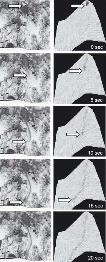
Fig. 11. Results of numerical simulation (right) compared with the observations (left) for the case 2 avalanche.
Artificial Avalanche Experiments
The chances of observing a falling avalanche in nature are extremely low. Together with safety problems, this is why observation data on natural avalanches are relatively scarce. There are only a few places where natural avalanches are observed regularly, such as the international avalanche release test sites at Ryggfonn, Norway (Reference GauerGauer and others, 2007), and Vallée de la Sionne, Switzerland (Reference Sovilla, Schaer and RammerSovilla and others, 2008). Researchers have also conducted numerous avalanche fall experiments with beads or foamed polystyrene instead of snow (e.g. Reference Hutter, Koch, Plüss and SavageHutter and others, 1995). Although such experiments can reproduce the dynamics of moving snow masses, they usually fail to reproduce erosion or deposition processes which are especially significant near obstacles.
In this study, we prepared a wooden artificial slope 5.4m long (Fig. 12a) and conducted several avalanche experiments with natural snow. Obstacles of various kinds can be installed at the bottom of the slope (Fig. 12b).

Fig. 12. Wooden slope for avalanche experiments: (a) photo, (b) draft with sizes.
The set-up parameters for numerical calculations are
snow density = 200kgm–3
adhesive force = 0Pa
inner friction angle = 24˚
plastic viscosity = 0.012Pa s
maximum time-step = 0.01s
mean particle spacing = 0.01m.
The following four types of avalanche experiment were conducted:
Slope-only without obstacles.
Stake row with 0.02m spacing.
Stake row with 0.04m spacing.
Notched board.
All stages of the experiments (start, falling, deposition) were thoroughly recorded with a camera and compared with the results of numerical simulations. For better reliability, every experiment was conducted twice.
Analyzing the falling stage (Fig. 13), which is common for all types of experiments, we noticed a small discrepancy in the shape and falling velocity of the avalanche at the very beginning of the experiments (1s). This can be explained by the fact that the snow block fallen from the container cannot be described as powder material initially, so the dynamics at the time of collision with the slope differs from the calculated behavior. The model limitations (e.g. ambiguity of the processes near the walls, or errors in measurements of the snow property in the experiments) may cause the discrepancy, though.

Fig. 13. Avalanche falling compared with the numerical calculations.
However, after 2s of the experiment the avalanche state became very close to that of numerical results, including the shape of the deposition cone in the lower part of the slope (Fig. 14).

Fig. 14. The case of a slope without obstacles: (a) avalanche deposition in the simulation and the experiment; (b) avalanche propagation graph; (c) forms of the avalanche body after 1, 2, 3 and 4s of falling.
When a row of narrowly spaced (0.02m) stakes is installed at the bottom of the slope, some snow is expected to be deposited above the stakes as has been successfully confirmed by both experiments and numerical calculations (Fig. 15). However, the MPS method results in graduate snow flowing through the gaps between the stakes until there is almost no snow on the obstacle. This problem still remains and is due to be studied in the future. We believe that including a change in snow property in the model may resolve the problem.
Fig. 15. The case of a slope with 0.02m spaced stakes: (a) avalanche deposition in the simulation and the experiment; (b) avalanche propagation graph; (c) forms of the avalanche body after 1, 2, 3 and 4s of falling.
In the case of a wider gap (0.04m) between the stakes, both experiment and calculations gave the same result: almost no snow remains on the obstacle (Fig. 16).
Fig. 16. Same as Figure 15, but with 0.04m spaced stakes.
In the case of the notched board obstacle (Fig. 17), we encountered a problem similar to that in the experiment with spaced stakes (Fig. 15) when the snow deposited on the obstacle gradually flows down (although quite slowly) from the edges. Therefore, an experimenter has to decide each time when to stop the calculation process.
Fig. 17. The case of a slope with a notched board obstacle: (a) avalanche deposition in the simulation and the experiment; (b) avalanche propagation graph; (c) forms of the avalanche body after 1, 2, 3 and 4s of falling.
Conclusions
The combined Bingham–dilatant fluid model with included erosion and deposition processes helped to resolve a number of tasks that could not be numerically resolved before. When this model was implemented, the reproduction of avalanches involving snow on slopes, avalanche stabilizing, shear strain dynamics and other processes became possible.
Despite some model limitations (e.g. ambiguity of the processes near the walls, and some randomness during the avalanche experiments), good reproducibility and agreement between field observations, results of several avalanche experiments and the numerical simulations were confirmed, proving that the MPS method is widely applicable for a variety of conditions. However, we believe that the snow property changing in time should be included in the MPS method to reproduce some specific cases (e.g. snow collisions) that will make this method even more reliable. Also, as a future prospect of the MPS method, more simulations and comparisons with avalanche data should be done to verify the model approach more definitely and to improve the model where discrepancies are observed.
Acknowledgements
We are grateful to I. Kamiishi (Snow and Ice Research Center, National Research Institute for Earth Science and Disaster Prevention, Nagaoka, Japan) for providing us with the avalanche pictures, without which this study would not have been possible.


