


Introduction
Rating equations are unquestionably the most widely used means of estimating unknown suspended sediment concentrations (Ĉ) and loads ![]() in glacier-fed and normal rivers alike. Their popularity lies in the apparent simplicity of their derivation and application. C is held to be a function of stream discharge (Q), and the relationship between measured values of C and Q is formulated as a regression model. The resulting equation is combined with measured values of Q to estimate unmeasured concentrations (Ĉ) directly and unmeasured loads
in glacier-fed and normal rivers alike. Their popularity lies in the apparent simplicity of their derivation and application. C is held to be a function of stream discharge (Q), and the relationship between measured values of C and Q is formulated as a regression model. The resulting equation is combined with measured values of Q to estimate unmeasured concentrations (Ĉ) directly and unmeasured loads ![]() as a time-referenced ĈQ product. A model which requires the use of only Q data to provide estimates of C and L is clearly highly suitable for practical purposes. On the other hand, such a model excludes reference to variations in sediment delivery (notably in relation to drainage shift, glacier motion, rainfall, and mass-movement events), and is thus an oversimplified representation of the process system. Whether the simple rating model remains, nevertheless, a valuable practical tool hinges upon the quality of the estimates it delivers.
as a time-referenced ĈQ product. A model which requires the use of only Q data to provide estimates of C and L is clearly highly suitable for practical purposes. On the other hand, such a model excludes reference to variations in sediment delivery (notably in relation to drainage shift, glacier motion, rainfall, and mass-movement events), and is thus an oversimplified representation of the process system. Whether the simple rating model remains, nevertheless, a valuable practical tool hinges upon the quality of the estimates it delivers.
The quality of rating equation estimates depends in part upon the extent to which the deterministic effect modelled by the fitted function exerts control upon variability in C (relative to stochastic effects and omitted deterministic effects), in part upon how well the data used to derive the rating equation fit the assumptions of the model applied, and in part upon how well conditions in the forecast period (the horizon) match those in the original derivation period (the origin). This paper extends previous evaluations of the quality of estimates from suspended sediment rating equations and transfer functions for the basin of Glacier de Tsidjiore Nouve, Switzerland (Reference Gurnell and FennGurnell and Fenn, 1984; Reference Fenn, Gurnell and BeecroftFenn and others, 1985), by examining the stability of rating relationships derived from the same basin for six different ablation seasons. The general question addressed here is that of temporal specificity: how good are estimates of C and L when simple rating equations are used beyond their frame of origin?
The Data Base
Table I details the sampling base of the six data sets examined herein. Suspended sediment concentrations were measured in units of mg 1−1 (1 mg 1−1 = 1 g m−3). Stream-flow discharges are expressed in units of 1 s−1( 11 s−1 = 1 × 10⁻³m3s−1). Scatter plots of C against Q for each year are shown in Figure 1. The data differ substantially from year to year. Full details of the site, and of the field and laboratory methods employed have been given in Reference Fenn, Gurnell and BeecroftFenn and others (1985).
Derivation of Rating equations: Technical Background
Rating equations are typically derived via the ordinary least-squares (OLS) regression procedure. The assumptions of the technique, and the consequences of violating those assumptions, are by now well known (e.g. Reference FergusonFerguson, 1977). Whilst those relating to the response between the dependent and the independent variables can be satisfied by careful experimental design, by partitioning and/or lagging cases as required and by adopting the correct functional form of model, those relating to the properties of the residuals are more difficult to satisfy.
Untransformed C-Q rating models are prone to yield residuals which are not normally distributed, are not homoscedastic and, in the case of glacier basins, are not serially uncorrelated. The log-log transform is frequently adopted as a joint solution to the first two of these problems. Since estimates of C, as opposed to log C are required, the log-log model is re-expressed via the usual back-transformation procedure as a multiplicative relationship between C and Q. The back-transformation introduces an
Table 1. The sampling base of the glacier de tsidjiore nouve data
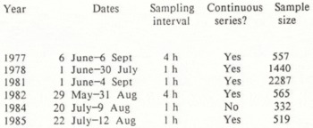
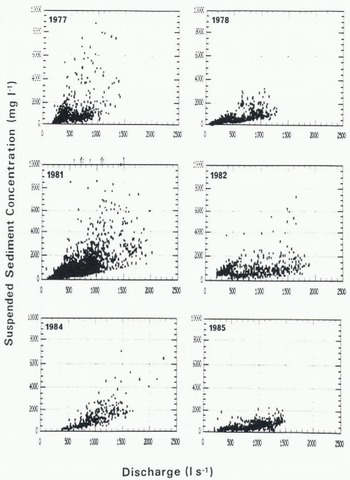
Fig. 1. Scatter plots of suspended sediment concentration against stream discharge for each of the six field seasons. The arrows on the 1981 plot indicate extreme values associated with outburst events:magnitude from left to right (in mg l−1), 11 124, 12 660, 18 025, 25 963, 13 830, 11 855, 12 901, 25 655, 70 774.
underestimation bias into predictions of C, however, since it yields the geometric as opposed to the arithmetic mean of the conditional distribution of C at any given value of Q (Reference FergusonFerguson, 1986). A correction factor (Bf) proportional to the standard error of estimate (s) of the log-log model reduces this bias (Reference MillerMiller, 1984; Reference JanssonJansson, 1985), (Bf = exp(s 2/2) for natural logs, exp(2.65s2) for common logs). The adjustment amounts to an upward, parallel shift of the rating curve on the log-log plot, and a higher, steeper curve on the arithmetic plot (Reference FergusonFerguson, 1986). The problem of true autocorrelation in the residual series (as distinct from quasi-autocorrelation resulting from the mis-specification of the model, the omission of important variables, and the presence of lags and/or changes in response) can be treated by the use of a generalized least-squares (GLS) model weighted by the serial correlation coefficient of the residual series. By turning the autocorrelation structure to advantage, a transfer function (TF) can be developed as an alternative to a regression equation (Reference Gurnell and FennGurnell and Fenn, 1984). Although preferable, this may be inconvenient, given the higher demands of developing a transfer function, or even a GLS regression equation, compared to an OLS regression equation. It is thus appropriate to evaluate the simple rating model in terms of its ability to deliver satisfactory estimates, as well as in terms of its statistical validity.
Ols Rating Models for the 6 Year Glacier de Tsidjiore Nouve Data
Inspection of the C–Q scatter plots (Fig. 1) indicates the need to transform each and every data set in order to stabilize the variance. The Box-Cox transformation search procedure (Reference Box and CoxBox and Cox, 1964) indicated the suitability of the log-log transform in all cases. The transformed scatter plots (Fig. 2) show the improvement which is achieved. The results from OLS regression applied to each data set (and to the combined multi-year data set) are given in Table II. Bias-correction factors calculated for each data set are also shown, together with the corrected coefficient in the multiplicative model. The Durbin Watson d statistic indicates that all models yield positively autocorrelated residuals, that is d < d L, Ρ < 0.01. Detailed investigation of the 1978 data set, involving lagging the series to the best match position, splitting the data into sections of constantresponse, testing the effects of air temperature and rainfall, and deriving discriminant ratings for rising and falling stage and ablation periods has established that the autocorrelation is of the truerather than the quasi type, and is likely to be an inherent property of this type of data (Reference Fenn, Gurnell and BeecroftFenn and others, 1985). We should therefore beware of the attendant effects on the coefficients and statistics of the models. The coefficients a and b will be statistically unbiased, but their standard errors are likely to be underestimated, as is the variance of the residual series and the R 2 statistic correspondingly inflated.
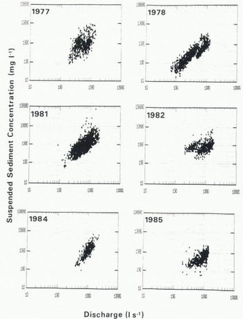
Fig. 2. Log-log scatter plots of suspended sediment concentration against stream discharge for each of the six field seasons.
Testing The Transferability of Rating Equations
Bearing in mind the reservations noted above, we can assess the degree to which a given rating model is likely to be temporally transferable by examining the stability of the coefficients of individual rating equations. An examination of the 95% confidence bounds of the regression coefficients that is, a ± 1.96SEa, and b ± 1.96SEb) indicates a minimal degree of overlap across the 6 year data set (Table II). The Chow test of equality of coefficients (Reference ChowChow, 1960) on the 6 year set results in rejection of an hypothesis of no difference in coefficients between years (F* = 195.4, Ρ 0.001). Allowing for the fact that standard errors (SEa, SEb) involved in the first test, and the error sums of squares (ESS) involved in the Chow test may both be artificially low, it would still appear reasonable to accept that the coefficients of the rating model of 1 year cannot be taken to be applicable in any other year with any degree of confidence. Inspection of the positions and slopes of the curves for each of the 6 years on the rating plot (Fig. 3) provides an unambiguous confirmation of this conclusion.
Table 2. Coefficients and statistics of ols rating equations
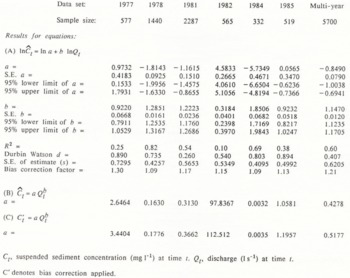
Ct, suspended sediment concentration (mg 1−1) at time t. Qt,discharge (1 s−1) at time t.
C′ denotes bias correction applied.
A similar picture emerges with respect to the stability of coefficients of rating models developed for partial periods of a single ablation season. The Chow test was applied in a comparison of coefficients of the whole 1978 data set against the coefficients of models for the June and the July data separately (F* = 3197.5), models for the pre-first flush and post-first flush periods identified in Reference Fenn, Gurnell and BeecroftFenn and others (1985) (F* = 3604.4), and models for each of the nine sub-periods of alternately rising and falling ablation which constituted the 1978 season (F* = 611.8). All F*values lie well above the critical value at p < 0.001.
It would appear reasonable to conclude from the above analyses that the sampling variability of the C–Q relationship is so great, on both year-to-year and within-year time-scales, as to preclude the transferability of a sample-rating equation to any other period save that which mirrors the conditions of the origin to a very high degree. This confirms the conclusions of Reference strem, Bridge and RannieØstrem and others (1967), Reference Ostrem, Jopling and McDonaldØstrem (1975), and Reference Fenn, Gurnell and BeecroftFenn and others (1985). The strict statistical implication is that the data from different years are derived from different populations. A glacio-hydrological translation of this, assuming that each glacier basin does have a population distribution, is that this distribution must be very large, and very heterogeneous, and that observations from a single-year sample only parts of the total population. This being so, there would appear to be some benefit in combining data from different samples as a means of approximating a population relationship for the basin.
A Multi-Year Rating Equation: Towards a General Model?
Combination of the 6 years of data for the Glacier de Tsidjiore Nouve basin results in a multi-year data base which includes the very different conditions associated with early season snow-melt periods,summer snowfall recession periods, rainfall events of varying intensity and duration, classic rhythmic diurnal cycles in flow and sediment transport, transient sediment flushes occuring independently of flow fluctuations, and extreme water/sediment outburst events; Q ranges from 70 to 2263 1 s−1 and C from 18 to 70774 mg l−1. The multi-year scatter plot benefits from a log-log transformation, although some degree of heteroscedastic behaviour remains (Fig. 4). The OLS rating model fitted to the multi-year data exhibits the familiar problem of autocorrelated residuals (Table II). Estimates from the multi-year model may accordingly lack precision (since OLS does not yield the minimum variance solution), but they are likely to be accurate. Since estimates of such quality may be acceptable inoperational practice, it is appropriate to evaluate the performance of the multi-year model in terms of the magnitude of error involved in its use as an estimating tool.
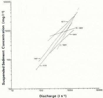
Fig. 3. Bias-corrected OLS-rating curves for the six ablation seasons.
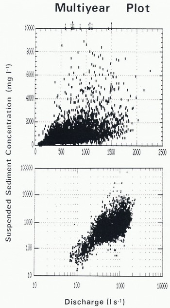
Fig. 4. Scatter plot (upper diagram) and log-log scatter plot (lower diagram) of suspended sediment concentration against stream discharge for the collected multi-year data set (n = 5700). The arrows on the upper plot refer to the extreme values identified in Figure 1.
Quality of Forecasts from Rating Equations
The success of the multi-year rating equation in estimating suspended sediment load in different years is now assessed in comparison with equivalent estimates obtained from each of the single season OLSmodels. For further comparisons, estimates are also obtained from a GLS model and from a transfer function (TF). The GLS model was derived from the 1978 data set via the Cochrane-Orcutt method (Reference Cochrane and OrcuttCochraneand Orcutt, 1949) as a means of handling the autocorrelation present in the residual series. The transfer function was developed from an arbitrary, as opposed to an optimally selected, 25 d period within the 1981 set via the Box-Jenkins method (Reference Box and JenkinsBox and Jenkins, 1970). The model was deliberately kept simple, in order that it could be used for making practical predictions. The constant was fixed at zero, and an equation containing only one coefficient was selected. The noise term used in the estimation phase was dropped when making predictions, on the grounds that zero is the expected value of the residuals. Reference Gurnell and FennGurnell and Fenn (1984) have described the procedures involved in developing the function.
Each equation was used to produce a series of estimated suspended sediment concentrations for the full duration of each of the six field seasons examined. These estimated concentrations (Ĉ) were then combined with the discharge data to produce an estimated load ![]() for each year, whilst the measured concentrations (C) were similarly used to produce a true load (L). The prediction equations used to calculate Ĉ are given in Table III. The OLS equations require only a discharge record to yield estimates of Ĉ, but the GLS and TF equations also require the provision of a starting value for C (C
0), since both involve a Ct-1, term. The starting values used in this analysis were not specially selected, nor were different selections attempted in order to achieve an optimum result; the starting value C0 was, in all cases, simply taken to be that value of C measured immediately before the start of the prediction period. Thereafter, estimated values of C (Ĉ) were used as valuesof C
t-1 to calculate forward. Only a single value of C0 thus needs to be measured in order to run the GLS and TF equations. Intermittent measured values of C can, of course, be fed in as values of C
t-1 to retarget the estimation as required.
for each year, whilst the measured concentrations (C) were similarly used to produce a true load (L). The prediction equations used to calculate Ĉ are given in Table III. The OLS equations require only a discharge record to yield estimates of Ĉ, but the GLS and TF equations also require the provision of a starting value for C (C
0), since both involve a Ct-1, term. The starting values used in this analysis were not specially selected, nor were different selections attempted in order to achieve an optimum result; the starting value C0 was, in all cases, simply taken to be that value of C measured immediately before the start of the prediction period. Thereafter, estimated values of C (Ĉ) were used as valuesof C
t-1 to calculate forward. Only a single value of C0 thus needs to be measured in order to run the GLS and TF equations. Intermittent measured values of C can, of course, be fed in as values of C
t-1 to retarget the estimation as required.
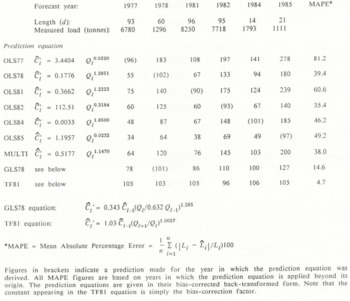
Each predicted load is expressed as a percentage of the corresponding measured load in Table III. The figures confirm, on a year-to-year time-scale, that an equation developed from a period of low sediment transport underestimates loads when it is applied to periods of higher sediment transport and vice versa, according to the disparity between conditions in the origin and the horizon (e.g. OLS85 badly underestimates load in all other years; OLS77 badly overestimates load in all other years). The figures in Table III show just how serious the under- or overestimation may be. The MAPE value provides a useful relative measure of the performance of each model as a predictive tool, enabling us to quantify the errors involved in applying a given rating equation beyond its derivation period. It is clear from the MAPE figures given in Table III that transferring OLS rating equations from one year to another leads to absolute errors of estimation in the order of 35–81%, averaging at 52%. The multi-year data model gives errors averaging 38%. The GLS78 model performs substantially better, yielding an average absolute percentage error of 15%. The transfer function, however, performs on a higher level altogther, giving a MAPE value of only 5%. The year-to-year transferability of what is in essence a very simple transfer function is remarkable. It raises the possibility that the structural form of the function has a sound physical basis. The stability of the structure and coefficients of transfer functions developed from different years thus require examination.
Conclusions
Ordinary rating equal ions change from year to year, and from period to period within a year. Their application in times other than those in which they were developed accordingly leads to substantial error in estimation of suspended sediment concentrations and loads. A rating equation developed from a multi-year data set improved upon the average performance of single-year models, but only to a limited extent. In contrast, GLS and TF models produced significantly better results. This is because these models calculate changes in suspended sediment concentration resulting from change in discharge, and because they address the autocorrelation structure in the C–Q relationship. Whilst the GLS andTF models are more difficult to develop than an OLS model, they are no more difficult to apply, in that they require only an initial measured value of C in order to run. The initial values used in these tests were not optimized but, since the value used for C0 is pivotal, the effects on final estimates of using different values of C0 require evaluation. The simple transfer function used here showed a consistent ability to estimate suspended sediment loads indifferent years with an absolute error margin of only 5%. We can conclude that the simple transfer function has been shown to be substantially more robust to temporal transference than OLS-rating curves. OLS-rating equations provide poor estimates of the suspended sediment load exported from glacierized basins when used beyond their frames of origin. Transfer functions appear to offer much greater promise in estimating suspended sediment transport in glacier melt-water streams. Figures in brackets indicate a prediction made for the year in which the prediction equation was derived. All MAPE figures are based on years in which the prediction equation is applied beyond its origin. The prediction equations are given in their bias-corrected back-transformed form. Note that the constant appearing in the TF81 equation is simply the bias-correction factor.
Table 3. Predicted suspended sediment loads as percentages of measured loads
Acknowledgements
The 1977 and 1978 sediment data were obtained during the tenure of a U.K. Natural Environment Research Council research studentship. Collection of the 1984 and 1985 sediment data was supported by grantsfrom Worcester College of Higher Education. The 1981 and 1982 sediment data were provided by I. Beecroft. Discharge data were provided by Grande Dixence S.A.


