


1 Introduction
The processes which contribute to the decrease in size of an iceberg can be discussed under three headings. The first concerns the action of surface waves. These bring warm water continually into contact with the ice, thus causing enhanced melting at the water line. This leads to the familiar undercut zones. As far as the author knows, only one quantitative experiment has been conducted which models this melting. Reference Martin, Josberger, Kauffman and HusseinyMartin and others (1978) measured the indentation produced in a block of ice placed in a wave tank. The vertical extent of melting in the ice above the water line was found to be about one and a half times the wave amplitude and that below the water line to be about one half the wavelength. Further experiments, at different wave amplitudes and wavelengths, would be interesting.
Associated with this wave-induced melting and the resultant undercutting of the ice, is the breaking-off of ice chunks to form bergy bits (Reference RobeRobe 1978). Such fragmentation of a berg decreases its size much more than the melting which causes it. This leads to the second category of iceberg deterioration: breaking. Breaking can result in a few very small pieces of ice, or an iceberg can break up into two, three, or possibly even more large icebergs; and there is a continuum of possibilities between these.
While breaking is important, especially if the iceberg is under tow, the total volume of ice remains virtually the same. A decrease in the amount of ice can only be achieved by melting. This is the third category of iceberg deterioration, and the one upon which we concentrate in this paper.
A tabular Antarctic berg can melt along the top, along the bottom, or at the sides. Near the coastline, melting along the top will be small because the atmospheric temperature is below the melting point of ice. Indeed, one of the results of the 1978–79 Norwegian Antarctic Research Expedition was that, south of about 66°S., melt rates at the upper surfaces of icebergs were less than the precipitation rates (Reference OrheimOrheim 1980). As an iceberg drifts (or is towed) further north, the surface melt rate will increase. If the atmospheric conditions of temperature, moisture, and wind speed above the iceberg were known, the heat transfer to the ice could be calculated (Reference Arya and PlateArya 1979) and hence the melt rate could be deduced. However, the presence of the ice changes the atmospheric conditions (cf. the fogs evocatively described by Reference WeeksWeeks (1980)), which makes calculating the melt rate difficult. Nevertheless, it seems reasonable to suppose that the melt rate at the upper surface will still be small compared to that at the bottom and the sides, which will now be in contact with relatively warm water.
Melting along the bottom of an iceberg has been the subject of three different studies. Reference Martin, Josberger, Kauffman and HusseinyMartin and Kauffman (1977) conducted a single experiment in which an ice block 0.45 m by 0.45 m by 0.1 m thick was placed on the surface of a 0.75 m-deep 37.6 0/00 NaCl solution maintained at 0°C. The ice extended to the sides of the tank and so there was no possibility either of melting at the side of the ice or of direct contact between the water and the atmosphere above the ice. The results of this time-dependent investigation were that for the 46 h of the experiment the melting along the bottom was well represented by
where z is the vertical co-ordinate of the bottom of the ice, t is the time since the initiation of the experiment and K ≈ 10-5m s-0.5. Extrapolating, with trepidation, this result to longer times, we might suggest that in the order of 100 mm of the base of an iceberg will melt in its first year.
A steady-state, rather than time-dependent, theoretical study has been presented by Reference GadeGade (1979). Unfortunately, however, he was unable to calculate the turbulent diffusivity associated with the convection under the ice. Rather, he compared his theory with observations of melting at the base of the Ross Ice Shelf (Little America V station) to determine the diffusivity coefficient. He thereby predicted a melting rate in the Antarctic of the order of 0.5 m a-1, although this value is, of course, heavily dependent on the Ross Ice Shelf data.
The preliminary results of an interesting experiment (Reference Russell-HeadRussell-Head 1980), in which ice measuring 1.0 m by 0.5 m by 0.25 m thick was placed on top of salt water in a tank 2.0 m by 1.2 m by 1.0 m high, are at variance with the results of Reference Martin, Josberger, Kauffman and HusseinyMartin and Kauffman (1977) and Reference GadeGade (1979). Russell-Head found that the melt rate at the base of the ice was comparable to that at the sides, and that, if the “ocean” was at 0°C and at 35 o/oo salinity, the melt rate was of the order of 102 m a-1. It is too early to comment reliably on the cause of the rather large differences between these and the earlier results.
The remainder of the paper is devoted to a discussion of melting along the side walls of an iceberg. A large part of our knowledge in this area comes from laboratory experiments on relatively small pieces of ice. The expectation is that if the important physical effects involved in the melting are properly modelled and correctly scaled, results for the melting of large Antarctic icebergs can be deduced. There is no doubt, however, that more observations in the Antarctic are needed in order to test some of the ideas which will be outlined below. The next section presents the convection patterns to be expected if the water surrounding the ice is either at a uniform density or incorporates a vertical density gradient. The final section discusses field data which may be compared with these predicted patterns.
2 Side-Wall Melting
(a) Uniform density surroundings
There have been a number of independent studies of a vertical ice wall melting into uniform surroundings, including those by Reference NeshybaNeshyba (1977), Reference GrcismanGreisman (1979), and Josberger (unpublished)Footnote *. Some of the results of Josberger's study with bubble-free ice between 0.5 and 1.2 m in length are neatly summarized in Figure 1, taken from his thesis. For oceanic temperatures and salinities, at the bottom of the ice wall there is a laminar flow with an inner layer in which the fluid motion is upward and an outer layer in which it is downward. The inner layer contains relatively light, dilute, cold water and the outer layer contains relatively heavy, salty, cooled water. Beyond a rather small distance, which Josberger estimates to be of the order of 0.5 m under typical Antarctic conditions, the inner layer becomes turbulent and the convection pattern consists of a turbulent boundary layer with solely upward flow. This boundary layer entrains ambient salty water and increases its thickness in the order of z 0.25, where z is the vertical length measured from the bottom of the turbulent layer. Due to the divergence between the downward laminar flow and the upward turbulent flow, there is a thin region of fairly strong flow towards the ice centred on the level at which the flow changes form.

Fig. 1 A sketch of the convection pattern produced by a vertical ice wall melting in uniform surroundings (reproduced from Josberger (unpublished))
Josberger measured the melt rate dx/dt at oceanic salinities as a function of ΔT ≡ T ∞ − T fp, where T ∞ is the far-field temperature and T fp is the freezing point of water at the far-field salinity. For ΔT ≤ 9°C, Josberger’s results are well represented by
where C ≈ 7.5 × 10⁻⁴ deg-1.6 mm5/4 s-1. This indicates that the melt rate increases with depth and that a mean melt rate, dX/dt, for a vertical wall of depth D can be defined by
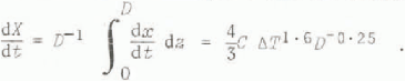
A few numerical values of the melt rate as a function of temperature difference and ice-wall length are given in Table I. It is interesting to compare the figures with the estimate of 50 to 100 m a1 suggested by Reference Morgan, Budd and HusseinyMorgan and Budd (1978) for the mean melt rate of Antarctic icebergs.
Table I The Mean Melt Rate, dx/dt, as A Function of the Temperature Difference ΔT and the Depth of the Vertical Ice Wall, D

The presence of bubbles in the ice, as observed in Antarctic glacial ice, may influence the melting. Bubbles increase the vigour of convection in the boundary layer by two distinct processes. First, the buoyancy difference between the layer and the ambient fluid is increased. Second, the bubbles drag up fluid by the added mass effect. However, in a series of experiments using ice with a C02 content of up to 5% by volume, Reference Huppert and JosbergerJosberger (1980) found that the melt rate was the same as that given by Equation (2.1) for the melting of bubble-free ice. Thus the quantitative effects of bubbles on the melt rate may be small.
(b) Stratified surroundings
In the Antarctic, as in most parts of the world's oceans, there is a vertical density gradient. The major cause of this density gradient in the Antarctic is salinity. Representative salinity and temperature profiles taken by Reference Foster and CarmackFoster and Carmack (1976) in the Weddell Sea are shown in Figure 2; the increase of salinity with depth, occasionally in a series of steps, is clearly evident.

Fig. 2 Profiles of temperature (T) and salinity (S) measured in the upper 400 m of the Weddel1 Sea (adapted from Reference Foster and CarmackFoster and Carmack 1976) (a) near the Scotia Ridge at the northern edge of the sea, and (b) near the turning point of the current gyre.
The convection pattern produced by ice melting in a salinity gradient cannot be the same as the turbulent upward motion already described. This is because an entraining upward flow would be carrying salt to levels at which the surroundings are less salty and hence lighter. The resulting buoyancy force would be of the wrong sign to allow the motion to continue. Instead, the motion is of the form displayed in Figure 3 Footnote *. This pattern was first reported by Reference Huppert and TurnerHuppert and Turner (1978), and was extended bv Reference Huppert and TurnerHuppert and Turner (1980) and Reference Huppert and TurnerHuppert and Josberger (1980). These papers present a more detailed discussion than we have room for here.
Next to the ice face there is a very thin layer of melt water flowing upwards. Beyond this layer there is a thicker outer layer flowing downwards. Due to the increase of salinity, and hence density, with depth the water in the outer layer, which has given up some heat in order to melt the ice, reaches a level of zero net buoyancy and flows away from the ice. This water is relatively colder and fresher than the inward flowing water just beneath it. This is because it has been cooled by both diffusion and the addition of melt water and, additionally, comes originally from a level of lower salinity. Double-diffusive convection thus occurs between the two counter-flowing layers, producing turbulence in these layers and in the outer boundary layer. It is because the outer boundary layer is turbulent that it entrains melt water from the inner boundary layer and eventually deposits it at a level not far from where it was formed. The heat transfer associated with the double-diffusive convection is responsible for the slight upward tilt of the interfaces apparent in Figure 3.

Fig. 3 Photographs of the convection pattern produced by a vertical ice wall melting in stratified surroundings:
(a) shadowgraph. Specific gravity at top 1.01 and at bottom 1.05. Temperature ≈ 20°C.
(b) using side lighting and ice made from water containing fluorescein dye. Specific gravity at top 1.00 and at bottom 1.03. Temperature ≈ 22°C. The light-coloured (fluorescein-enriched) water contains melt water, while the dark-coloured water is pure ambient water.
From an evaluation of the buoyancy forces acting on fluid parcels undergoing the motion described above, it is clear that the thickness of each layer will be of the form
where: ρ(T,S) is the density as a function of temperature T, and salinity. S; the subscripts w and ∞ indicate evaluation at the ice wall and in the far-field respectively; and dp/ds is the vertical density gradient due to salt. The constant 0.65 is determined experimentally. Its value is less than unity because there is a horizontal temperature gradient in the downward-flowing outer layer and thus some of the fluid particles in the boundary layer are not cooled to Tw . For numerical evaluation of (2.3) little error is incurred by replacing Tw by Tfp , the freezing point at the far-field salinity. Figure 4 presents in graphical form the data from experiments reported by Reference Huppert and TurnerHuppert and Turner (1980) and Reference Huppert and TurnerHuppert and Josberger (1980). Included in the figure is the relationship (2.3), which is seen to fit the experiments for a range of density gradients which spans almost two orders of magnitude.

Fig. 4 The layer thickness per unit specific gravity difference as a function of the vertical specific gravity gradient, from experiments of a vertical ice wall melting into a salinity gradient reported by Reference Huppert and TurnerHuppert and Turner (1980) and Reference Huppert and TurnerHuppert and Josberger (1980). ρ o is the mean density of the ambient water.
3 Field Observations
Detailed observations on melting icebergs or oceanographic properties in the vicinity of icebergs are unfortunately rare. The data of Reference Foster and CarmackFoster and Carmack (1976) displayed in Figure 2 indicate a stepped structure which might be due to the melting process described in the previous section. Evaluation of the thickness of each layer as predicted by Equation (2.3) leads to the results presented in Table II. The agreement between the layer thickness actually observed in the upper 100 m in the centre of the Weddell Sea and that predicted is quite good. A series of layers is rather more difficult to discern in the more northern observations; this might be due to the paucity of icebergs in the vicinity. Below 100 m in the central region, the stratification is virtually zero and the convection pattern should be of the type described in section 2(a).
Table II The Vertical Density Gradient Deduced From Foster and Carmack (1976) and the Predicted Layer Thicknesses According to Equation (2.3)

Further data come from some measurements in fjords. Reference Piekard and StantonPickard and Stanton (1979) have compiled a detailed description of the many Pacific fjords found in Alaska, Canada, Chile, and New Zealand. Their survey indicates that those fjords with glaciers at their heads, when contrasted with those without, tend to have a stepped salinity structure and a positive dissolved oxygen anomaly. The latter could be explained by some of the air which is trapped in the glacier flowing horizontally with the melt water rather than rising to the surface.
Finally, S.S. Jacobs (private communication) has made some measurements near the terminus of the Erebus ice tongue. He found a well-developed step structure between about 75 and 225 m with a layer thickness of approximately 20 m. This is in accord with the value calculated from Equation (2.3). Further details will appear in a paper in preparation by S.S. Jacobs, H.E. Huppert, G. Holdsworth and D.J, Drewry.
It is clear from this short catalogue that theory and laboratory observations greatly outnumber field data. The time therefore seems ripe for a series of ocean measurements to confirm, or bring into question, our present understanding.
Acknowledgements
It is a pleasure to thank my colleagues Professor J. Stewart Turner and Dr E.G. Josberger for the many stimulating discussions which we had about icebergs. My work is supported by the Ministry of Defence (Procurement Executive).


