


Introduction
Calving (both the total volume calved as well as the frequency and size of calved blocks) plays a critical yet not well understood role in glacier mass balance (Reference Kaser, Cogley, Dyurgerov, Meier and OhmuraKaser and others, 2006), glacier dynamics (Reference Benn, Warren and MottramBenn and others, 2007; Reference Nick, Vieli, Howat and JoughinNick and others, 2009; Reference Amundson and TrufferAmundson and Truffer, 2010) and fjord circulation processes (Reference Motyka, Hunter, Echelmeyer and ConnorMotyka and others, 2003; Reference Amundson, Fahnestock, Truffer, Brown, Lüthi and MotykaAmundson and others, 2010). Calving and submarine melt account for nearly all of the mass loss from the Antarctic ice sheet (Reference RignotRignot and others, 2008) and half of the mass loss from the Greenland ice sheet (Reference Van den BroekeVan den Broeke and others, 2009). Calving and submarine melt can also dominate the mass loss for marine-terminating alpine glaciers, resulting in a substantial contribution to eustatic sea-level rise that is primarily due to their dynamic instability (Reference MeierMeier and others, 2007). The few studies that have attempted to separate calving from submarine melt suggest that they are both important contributors to mass loss (Reference Motyka, Hunter, Echelmeyer and ConnorMotyka and others, 2003, Reference Motyka, Truffer, Fahnestock, Mortensen, Rysgaard and Howat2011; Reference Rignot, Koppes and VelicognaRignot and others, 2010). Despite the importance of calving, measurements of the calving process are difficult and introduce significant uncertainties into mass-balance and sea-level rise estimates primarily because of the stochastic nature of the calving process and multiple time and spatial scales involved (Reference Kaser, Cogley, Dyurgerov, Meier and OhmuraKaser and others, 2006; Reference BassisBassis, 2011). Passive underwater acoustics presents a new method for observing calving to both help understand the underlying processes and detect and measure calving events.
Underwater ambient sound in most oceanic environments has been measured and characterized for navigation, military and scientific as well as other reasons (Reference Knudsen, Alford and EmlingKnudsen and others, 1948; Reference WenzWenz, 1962; Reference UrickUrick, 1984; Reference Dahl, Miller, Cato and AndrewDahl and others, 2007; Reference Carey and EvansCarey and Evans, 2011). Microseisms and wave–wave interactions dominate infrasound frequencies (Reference Kibblewhite and WuKibblewhite and Wu, 1989) supplemented by earthquakes and explosions. Slightly higher infrasound frequencies (5–20 Hz) correlate best with wind speed (Reference NicholsNichols, 1987). In many environments, anthropogenic sounds dominate frequencies from 10 to 150 Hz, especially near shipping lanes (Reference RossRoss, 1987). At slightly higher audible frequencies (400– 20 000 Hz), wind dominates the ambient sound in most oceanic environments, primarily due to bubbles and spray associated with waves (Reference Medwin and BeakyMedwin and Beaky, 1989). Every oceanic environment is slightly different, and anomalous ambient sounds in an environment can offer clues to processes specific to that environment. Scientists have studied the ambient sounds of arctic sea-ice environments, initially because of military interest in the sub-sea-ice environment, although interest has expanded over the last few decades due to environmental and climate change questions (Reference MilneMilne, 1967; Reference Lewis and DennerLewis and Denner, 1988; Reference Langhorne and HaskellLanghorne and Haskell, 1996). Several studies have explored global ice-generated hydroacoustics at low frequencies (Reference Chapp, Bohnenstiehl and TolstoyChapp and others, 2005; Reference Talandier, Hyvernaud, Reymond and OkalTalandier and others, 2006; Reference MacAyeal, Okal, Aster and BassisMacAyeal and others, 2008). Very few observations, however, have been made in fjords with active glaciers (Reference Pettit and NystuenPettit and Nystuen, 2009), yet there is much potential for using ambient underwater sound to study processes such as calving ice, melting ice, freshwater upwelling or glacier motion.
We present the first spectral analysis of passive underwater acoustic signals from a subaerial calving event and the subsequent mini-tsunami and seiche that occurred on 2 May 2008 at Meares Glacier, south central Alaska, USA, in order to provide a foundation for future research or monitoring of processes at the ice–ocean boundary. The calved block was estimated to be 10 m tall (judged relative to the height of the cliff), of similar width and an unknown thickness (but most likely <10m based on observations of icebergs in the fjord). It created a noticeable mini-tsunami that traveled along and across the fjord, reflected multiple times from the valley sides, and created a seiche. In addition to glaciological and oceanographic interest in the physical processes associated with calving events, calving events also present natural sounds somewhat similar in magnitude and character to many of the anthropogenic sounds (such as explosions or pile driving) that concern marine biologists (Reference Popper and HastingsPopper and Hastings, 2009; Reference Dunlop, Cato and NoadDunlop and others, 2010).
The calving event we characterize here is a typical event of moderate size for this glacier. It was large enough to create a mini-tsunami and seiche that jostled and moved all the icebergs and brash ice in the forebay, including our boats, but it was not unusually large or unique in any other way, except that it occurred after a period of several hours of little calving activity. The calmness of the fjord preceding the event allows us to distinguish sound related to this specific calving event from that related to other processes within the fjord, such as wave action from wind or other calving events, wind-induced movement of icebergs, or overturning of larger bergs. Many of the characteristics we present here appear to be common to other calving events, just not as distinguishable in the data.
To summarize the sequence of events detailed in this paper, the first sound to arrive is a sudden low-frequency event with energy primarily in the infrasound range (1–20 Hz), but also including low-frequency audible sounds (20–100 Hz). After several seconds there is a sudden increase in intensity for 1 s at frequencies between 20 and 80 Hz that we associate with the fracture and detachment of the calving block. This is followed after <1 s by a sharp peak at ~400 Hz (with some energy at higher frequencies as well), which we interpret as the block impacting the water surface. Following this peak, a gradual increase in energy at high (10 000–20 000 Hz) and ultrasonic (20 000–40 000 Hz) frequencies ultimately persists with varying intensity for over 10 min which is the result of the mini-tsunami and seiche activity. This persistent high and ultrasonic frequency sound is accompanied by high-intensity infrasound that is likely due to pressure fluctuations in the fjord due to wave interference during the seiche.
Meares Glacier Setting
Meares Glacier (Fig. 1) originates from the Chugach Mountains and lies one valley to the west of Columbia Glacier which has been well studied. Meares Glacier empties into Unakwik Inlet, which connects to the Gulf of Alaska through Prince William Sound. Very little published research has been conducted on Meares Glacier, although it is noticeably, if slowly, advancing because it is overriding old growth forest (Reference Trabant, March and MolniaTrabant and others, 2002). Unakwik Inlet is known anecdotally to be often ice-free or nearly ice-free, making it ideal for accessing the glacier terminus.

Fig. 1. Map of Meares Glacier and Unakwik Inlet, Alaska, which opens into Prince William Sound. Inset shows location of Unakwik Bay (blue star) within Alaska. The red star identifies the location of the hydrophone deployment (61.149˚ N, 147.53˚ W) ~300m from Meares Glacier terminus.
According to Brown and others (1982), the water depth at the terminus in the center is 63m (average 31 m), the subaerial ice-cliff height averages 59 m, the width of the calving face is 1440 m and ice at the terminus moves with an average speed of ~1kma–1. Reference Brown, Meier and PostBrown and others (1982) cite it as a slightly retreating glacier in 1977; however, terminus position has not changed substantially since 1977. With these observations, we consider it a stable terminus on a multi-decadal scale. As a stable terminus with ice velocity of ~1kma–1, it therefore produces an average of ~3.5×10⁵ m3 d–1 total iceberg and submarine meltwater volume. There are few observations of frequency–size distributions for calving and most are for large events or from iceberg distributions (Reference BahrBahr, 1995; Reference Savage, Crocker, Sayed and CarrieresSavage and others, 2000); however, an inverse power-law or fractal relation is considered most probable in which small events are very frequent and large events are infrequent. Considering that the size of this event is 1/500 of the daily ice flux and several hundred calving events per day of all sizes are not unusual, we consider this event to be small enough to be commonly occurring, but large enough to affect the fjord by causing a substantial seiche.
Unakwik Inlet is long and narrow with steep valley walls, although narrow beaches line the water edge near the glacier (more on the western side of the inlet than the eastern side). The glacier terminates just up-valley from a right-angle turn in the valley. This geometry creates an ideal situation for multiple reflections of the mini-tsunami created by the iceberg before the energy dissipates fully. The interference of these waves leads to a seiche in the forebay.
The speed of sound in water is determined predominantly by the temperature and the salinity (Reference MedwinMedwin, 1975). We do not have conductivity–temperature–depth (CTD) profiles for Unakwik Inlet; however, we do for several other glacial fjords in the Gulf of Alaska. All our CTD measurements show a similar pattern to that found by Reference Motyka, Hunter, Echelmeyer and ConnorMotyka and others (2003) in which a surface layer of cold fresh water lies on top of warmer saltier oceanic water. This results in a sound speed of ~1450ms–1 in the near-surface layer increasing to ~1470ms–1 near the bottom. This typical stratified structure of glacier fjords reduces the effectiveness of a sound channel (wave guide), such as the sound fixing and ranging (Sofar) channel, which is common in many other oceanic environments.
Data Collection and Analysis Methods
On 2 May 2008 we approached the center of the terminus to within 300m of the ice cliff in a dinghy (61.14835˚ N, 147.53149˚ W). Our access boat was anchored at ~1km from us with its engines and sonar turned off. During our data collection, we minimized sound related to the boat and the dinghy as much as possible. The glacier forebay consisted of small patches of brash ice, but no larger icebergs, and the glacier calving activity was generally quiet. It was near high tide. There was a very light drizzle with no measurable wind. When in position, we lowered two hydrophones into the water, one at 30 m depth and one at 16 m depth.
At 30 m depth we deployed a Benthos AQ-18 hydrophone (omnidirectional with sensitivity –171±1.5 dB reV μPa–1 over 0.1–10 000 Hz, using a preamplifier 26 dB) and at 16m depth we deployed a Seaphone SS03-10 (omnidirectional with sensitivity –168±1dB reVμPa–1 over 1000–30 000 Hz, using a preamplifier 25 dB; this system also includes adjustable amplification 0–30 dB, set to 0 dB for observations discussed here). Outside their stated range, the sensitivity varies by more than ~±1.5 and directionality may be altered, but the qualitative results are still valid. We primarily present data from the Benthos hydrophone here; the Seaphone produced qualitatively similar results. We recorded hydrophone output at 88 200 Hz sampling frequency to a flash drive using a TASCAM HD-P2 portable two-channel recording system. The TASCAM recording system includes additional amplification which was set to 32.3 dB for the recordings presented here, allowing us to make full use of the dynamic range of the recording system. It also has a speaker, allowing observers to correlate submarine signals (arriving first) with subaerial signals and visual observations. We recorded visual observations using a camera (when possible) and field notebook and linked them to the digital recordings using the recording system’s built-in file-marking system.
We observed and recorded several calving events during ~2 hours of observations, all of which show similar spectral characteristics. We focus our analysis here on a single event because this event occurred during a period when other ambient sound in the fjord was at a minimum.
We calculate sound pressure levels (SPL) using the standard methods for underwater sound (e.g. Reference MedwinMedwin, 2005). The voltage measured is directly proportional to the sound pressure; therefore, standard spectral density analysis on the time-domain waveform results in a power spectral density in units of μPa2 Hz–1. We calculate the SPL in dB re 1μ Pa2 Hz–1 as
where ![]() is the power spectral density for frequency band f
m. We processed the data using standard spectral analysis techniques. We used a combination of 8132-point (213) fast Fourier transform (FFT) spectrograms (most of what is shown here) along with 1024-point (210) and 131 072-point (217) FFTs to trade off time resolution with frequency resolution. We used the unfiltered dataset for the bulk of the spectral analysis. For the low-frequency time-domain analysis, however, we used low-pass and bandpass Butterworth zero-phase (acausal) filtering.
is the power spectral density for frequency band f
m. We processed the data using standard spectral analysis techniques. We used a combination of 8132-point (213) fast Fourier transform (FFT) spectrograms (most of what is shown here) along with 1024-point (210) and 131 072-point (217) FFTs to trade off time resolution with frequency resolution. We used the unfiltered dataset for the bulk of the spectral analysis. For the low-frequency time-domain analysis, however, we used low-pass and bandpass Butterworth zero-phase (acausal) filtering.
In water, high frequencies attenuate faster than low frequencies; therefore, the spectral characteristics of a sound source will be modified based on the distance to the source and frequency content of the sound (e.g. Reference MedwinMedwin, 2005). At 1000 Hz, attenuation is ~0.03 dBkm–1 in sea water (for fresh water it is <0.001 dB km–1). For 30 000 Hz the attenuation in sea water is ~10 dB km–1 (1 dB km–1 for fresh water). Considering our proximity to the calving source, we consider this attenuation negligible for all but the highest frequencies. At 30 000 Hz, we are likely underestimating true SPL by up to 10 dB. Because this is small compared with our signal and the exact source location for high-frequency content is distributed across the fjord, we do not correct for this in the data presented below.
Results
Figure 2 shows the pre-calving quiescent period, the calving event and the first 70 s of the mini-tsunami and seiche wave propagation and reflection. Figure 2a and h show the time-domain waveform for the event. Figure 2b and i show ΔSPL, the difference in SPL from that averaged over a quiescent period (4.4–6.0 s). This emphasizes the spectral anomaly produced by the calving event. Figure 2c and j show the total SPL in the 6–8 Hz infrasound band (note that the quiescent period is too short to provide a background SPL for the infrasound band), while Figure 2d–g show the ΔSPL for various frequencies. For simplicity of terminology, we use infrasound when discussing 1–20 Hz signals, low frequency when discussing 20–100Hz signals, mid-frequency when discussing the 200–600 Hz signals, high frequency when discussing the 10 000–20 000 Hz signals and ultrasound when discussing signals of 20 000 Hz. Within the infrasound, the 6–8 Hz band is the only one that shows correlation with this calving activity; therefore, Figure 2c and j show just this band and our analysis is focused on this band. The recorded data start ~10 s before the visible falling of the calved block. The timing of events stated here is approximate and results from correlating peaks in amplitude across multiple frequency bands and using the raw and filtered time-domain waveforms, rather than using arrival times in any specific band because of the acausal filtering process, which can cause filtered waveforms to show activity slightly before the event. In general, the higher the frequency of the event described, the more accurately we can pick the timing.
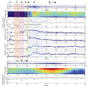
Fig. 2. The recorded event as: (a) the time-domain waveform of the first 40 s; (b) the spectrogram for waveform shown for ΔSPL calculated with 8192-point FFT in dB (re 1μPa2 Hz–1); (c) the total SPL for the 6–8 Hz band; (d–g) the ΔSPL at 30, 400, 11 000 and 35 000 Hz, respectively; (h) the time-domain waveform for the second 40 s; (i) the spectrogram of waveform in (h) for ΔSPL calculated with 8192-point FFT in dB (re 1 μPa2 Hz–1); and (j) the total SPL for the 6–8 Hz band. The vertical scale for the time-domain waveforms (a–h) is relative to the maximum dynamic range of the digitizer. Note that the consistent minimum in signal near 20 000 Hz is most likely due to the specific hydrophone response in that range (this is above the hydrophones ‘level’ response range).
Based on the spectral characteristics, the calving event can be divided into six phases.
Small event at 1.2 s
In Figure 2a, a small (perhaps 1 m3) ice block falls at ~1.2 s from the start of the recording. This small event only produces measurable sound at frequencies lower than ~1000 Hz. From seismic data, Reference Neave and SavageNeave and Savage (1970) suggest that ~30 Hz is a typical frequency for an ice fracture event, which, for this event, appears as a spike in Figure 2d. This occurs nearly simultaneously with a spike near 400 Hz, which we interpret as the sound of the ice block hitting the water based on our observations from numerous calving events. We observed no wave action subsequent to this event and there is no high-frequency content shown in Figure 2f and g. Figure 2c shows a peak in the infrasound band at ~2.5 s. This is significantly after the event at 1.2 s; therefore, we cannot confirm that the two events are related.
Phase 1: quiescent period
The period between the 1.2 s event and the main calving we call the quiescent period. The time between 4.4 and 6.0 s is the quietest time we observed within this period and we use the background ambient sound level during this time to highlight the details of the calving event. The SPL spectrum for the quiescent period is shown in Figure 3. There is one large peak at ~3500 Hz and another smaller peak at ~7500 Hz. According to Reference Pettit and NystuenPettit and Nystuen (2009), the peak at ~3500 Hz is due to bubbles forming in the water from the melting of glacier ice, which contains pressurized air in its pore space. The peak at ~7500 Hz we interpret as the light rain that was falling, based on analysis of similar observations by Reference NystuenNystuen (2001). Our analysis of the calving event does not show significant variation at these frequencies; therefore, these frequencies do not play a role in our analysis.
Fig. 3. The spectrum of SPL (dB re 1μPa2 Hz–1) for the quiescent period (4.4–6.0 s) using an 8192-point FFT analysis.
Phase 2: very low- (infrasound) and low-frequency onset
As shown in Figure 2c and d, at ~6.5 s a low-frequency rumble begins. This rumble contains energy over a broad frequency range less than 100 Hz. During this onset period, however, the SPL of the infrasound band (6–8 Hz) increases in intensity twice as much as the increase in intensity of the low-frequency band (20–100 Hz). There is no significant mid-, high- or ultrasonic-frequency content.
Phase 3: low-frequency pre-calving activity
At ~8 s, the low-frequency content (Fig. 2d) begins to increase in intensity, with a sudden increase at 8.9 s. This high-intensity low-frequency sound persists for ~0.7 s before decreasing again suddenly at 9.6 s to a similar SPL as at 8.9 s. This low frequency is difficult though not impossible to detect through the air by the human ear or through the transfer of the signal from the water into subtle vibrations in the floor of the dinghy. Our observer logs noted a number of low-frequency rumbling events, not all of which were associated with calving events. The infrasound band (Fig. 2c), on the other hand, shows only a modest increase during this time. Finally, during this period, there is still negligible sound emitted above ~100 Hz.
Phase 4: mid-frequency block impact
At 10.27 s there is a sudden increase in energy at mid-frequencies (from 100 to 600 Hz; Fig. 2e). Immediately following this, at 10.35 and 10.38 s the high- and ultrasonic-frequency bands respond, along with a smaller response in the low-frequency band. Based on our visual field observations, we associate these events with the impact of the block on the water (mid-frequency energy) and the initial splash of the water in response (high and ultrasonic frequencies). The response to the initial impact and splash lasts <0.5 s and is followed quickly by several additional smaller blocks falling, particularly at 10.9 s The mid-frequency shows a second peak at 11.3 s, which is a secondary calving event (a smaller block than the first, but still fairly large) impacting the water; this may be associated with a low-frequency peak at 10.4 s, as the fracture of this secondary block.
Phase 5: block oscillation in water
The high- and ultrasonic-frequency sound levels begin increasing after the calved block impacts the water and they reach a peak nearly 3 s later at 13.18 and 13.35 s. During this period, our field observations suggest that the block penetrates into the water until buoyancy forces cause it to return to the surface; we interpret the peak in high and ultrasonic frequencies to be the spray and wave action produced when the block returns to the surface the first time. The block then continues to oscillate due to buoyancy, but its oscillations are significantly damped after the first rebound, such that it is difficult to distinguish the second and third oscillations from other wave action. For these first ~5 s after the block impacts the water, the low and mid-frequencies stay relatively high before dissipating and returning nearly to pre-calving levels. These lower frequencies then remain at low intensity levels throughout the remainder of the event. The 6–8 Hz infrasound signal, however, does not dissipate. The infrasound has a broad peak between 11.5 and 12.1 s, which corresponds to the time that the block is at its deepest in the water (~11.75 s).
Phase 6: mini-tsunami and seiche action
At approximately 18 s, the iceberg motion dissipated, low-and mid-frequency ΔSPL dropped and we observed in the field that the iceberg had split into several smaller pieces. When a calved block is sufficiently large, the oscillation of the block in the water will create a mini-tsunami which radiates in all directions. We observed this mini-tsunami as it moved our dinghy farther from the glacier terminus. The mini-tsunami also traveled laterally along the ice front in both directions, reflected off the valley walls and returned to the center, where we observed in the field the constructive interference of the waves causing turbulence in the water and collisions among the small icebergs and brash ice left after the calving event. Figure 2b shows multiple periodicities (primarily at 1–2 and 6–7 s) in intensity (warmer colors) for the high- and ultrasonic-frequency sound levels that may be related to wave interference patterns. At 62 s, the constructive interference of the rebounded waves is near its peak; there is a significant increase in ultrasound energy starting at 55 s and lasting until 70 s (shown as red in Fig. 2i). There is a corresponding increase in the 6–8 Hz infrasound SPL (shown in Fig. 2j). These signals remain at levels significantly higher than the quiescent period for ~10 min, despite the lack of calving events during that time (some small blocks fell, but none large enough to affect the whole fjord).
Discussion
Phases 2–5 of this calving event occurred within 10 s, followed by the mini-tsunami and seiche activity which continued at significant levels for ~60 s and then slowly dissipated over the next ~10 min. The rapidity of these events, the limitation of having data from a single hydrophone and the difficulty of observing quantitatively the simultaneous processes in the water, ice and air make it challenging to confirm the physical processes underlying each phase of the event. Using related ocean acoustic and seismic studies with simple physical models, however, we deduced a possible sequence of events (each shown in Fig. 4 and discussed in more detail below):
Fig. 4. A diagram of each of the phases, showing one possible interpretation of the data.
Phase 2 – the infrasound signal has a sudden onset, accompanied by some energy in the low-frequency range. Although signals in this frequency band may be related to water resonating in a crevasse, because of its sudden nature we interpret this as a sudden movement of the glacier such as a basal slip event. This event caused instability in the incipient calving block.
Phase 3 – the new geometry of the incipient calving block induces stress concentration at the tip of the crevasse behind the block. The crack propagates, leading to detachment of the block. The detachment of the block induces further stress changes in the surrounding ice, leading to multiple small blocks detaching shortly afterwards.
Phase 4 – the primary block falls through the air, impacting the water, followed shortly by multiple small blocks. The impact produces a loud sound in the audible range.
Phase 5 – the block oscillates in the water, beginning with one large-amplitude oscillation. The impact and initial oscillation induce stress within the block that may fracture it into several smaller blocks, which dampens the subsequent oscillations.
Phase 6 – the oscillations produce a mini-tsunami which radiates in all directions, then rebounds off the terminus ice cliff and the valley sides. The rebounded waves interfere with each other, creating an interference pattern that has characteristics of a seiche.
Many aspects of this calving event are common to all of the subaerial calving events we observed. Variations in the size of the block, the height from which it falls, the brash ice cover in the fjord, the geometry of the glacier and fjord and other conditions will alter the intensity of the sounds and the magnitude of the mini-tsunami.
Phases 2 and 3: initial infrasound and low-frequency events
As mentioned earlier, our field observations and the acoustic recordings suggest that many calving events begin with an infrasound and low-frequency rumble. Further, these rumbling sounds also occur regularly without the production of an iceberg, suggesting that they are related to the dynamics of the glacier near the ice–ocean interface (such as basal sliding or release of subglacial water).
Within the infrasound band we studied (Fig. 2c), the 6–8 Hz range is significantly better correlated with the calving event than other measured infrasound signals from ~3 to ~20 Hz. Based on previous work by other researchers, there are three most likely sources for this precursory infrasound activity: (1) basal slip (i.e. movement along the fault at the ice–bed interface); (2) resonance of water movement in conduits, cracks and crevasses within the ice; and (3) wave–wave interaction within the fjord.
Reference QamarQamar (1988) found a linear relation between calving events and the duration of 1–2 Hz frequency seismicity at Columbia Glacier, Alaska, but did not detail the mechanism through which the calving event produces such a signal. It is possible, however, that a similar source is creating the infrasound signals we observe. Several other studies, including Reference Métaxian, Araujo, Mora and LesageMétaxian and others (2003), Reference O’Neel and PfefferO’Neel and Pfeffer (2007) and Reference West, Larsen, Truffer, O’Neel and LeBlancWest and others (2010), suggest that low-frequency seismic signals (<15 Hz) are related to movement of water through cracks, crevasses and conduits. In particular, Reference West, Larsen, Truffer, O’Neel and LeBlancWest and others (2010) detect events that begin with a higher-frequency signal (20–35 Hz) followed by a lower-frequency signal (1–15 Hz). They interpret this as a fracture in the ice followed by a flush of water through the new fracture. Alternatively, the infrasound signal may arise directly from a slip event at the bed (Reference Anandakrishnan and BentleyAnandakrishnan and Bentley, 1993; Reference Walter, Clinton, Deichmann, Dreger, Minson and FunkWalter and others, 2009). In our situation, the infrasound signal has a sudden onset (shorter than the FFT window size necessary to detect it) that precedes the significant activity at 20–100 Hz (which begins at 8.5 s; Fig. 5a). Because of the sudden onset, we interpret a basal slip event as the most likely source, as both wave–wave interaction and water movement in cracks are slow processes that would create an emergent signal. With the limited data available, however, we cannot distinguish unambiguously among these sources for the infrasound.
Fig. 5. A detailed look at the onset of the calving event in time domain at lower frequencies. (a) 6 s of the time-domain waveform bandpass filtered 20–100 Hz (the band associated with ice fracturing); (b) 0.3 s of the time-domain waveform bandpass filtered 200–600 Hz (the band associated with the impact of the block on the water). The vertical scale for the time-domain waveforms is relative to the maximum dynamic range of the digitizer, as discussed in text.
Figure 5a shows filtered time-domain waveforms for the low frequency (20–100 Hz) during the onset of the calving event. Figure 5a shows a low-frequency low-amplitude emergent event starting at ~6.5 s (coincident in time with the infrasound onset) that dissipates again until a sharper onset event occurs at 8.5 s. The amplitude in this frequency band increases further between 9.0 and 9.6 s. Several studies of seismic activity on glaciers suggest that ice fracture and crevassing produces seismic energy with a frequency that depends on the geometry of the crack, but is typically in this 20–100 Hz range (Reference Neave and SavageNeave and Savage, 1970; Reference Walter, Deichmann and FunkWalter and others, 2008; Reference West, Larsen, Truffer, O’Neel and LeBlancWest and others, 2010).
We suggest that this pattern of infrasound first (due to a basal slip event) and low frequency second (due to fracturing) indicates that the calving event is triggered by a sudden movement of the glacier due to basal slip. This movement generates a seismic signal in the ice and rock in addition to the infrasound signal in the water and causes the incipient calving block to become unstable. This may be the same signal as recorded by seismographs near other calving glaciers; however, Reference Walter, O’Neel, McNamara, Pfeffer, Bassis and FrickerWalter and others (2010) associate this seismic frequency band with water movement in cracks. Movement of water in crevasses is less likely as the cause of the infrasound we observe, because water movement typically would be an emergent and longer-lasting signal.
Following the infrasound trigger, a possible sequence of events is that the activity between 8.5 and 8.9 s is the primary fracturing activity that detaches the block from the glacier. At 8.9 s, the block begins to slide downward. During the initial part of the fall, the block remains in contact with the ice, similar to shearing on a fault. At 9.6 s the block is no longer in strong contact with the ice as it falls (due to the shape of the ice cliff and of the calved block).
Phase 4: impact of block with water
Figure 5b shows the time-domain waveform for the 200– 600 Hz band during the impact of the block with the water (phase 3). The ΔSPL associated with this is shown in Figure 2e. Both show a strong signal at 10.27 s. Based on a comparison of field observations of the subaerial and submarine signals of the event, we interpret the spike at 10.27 s as the impact of the block on the water. During any calving event, this impact is typically the loudest sound in the audible range. This event is no exception, as shown in Figure 2e.
Phase 5: oscillating iceberg
The iceberg has a certain amount of kinetic energy when it impacts the water surface. This energy will allow the iceberg to penetrate into the water column and initiate buoyancy-driven oscillations. The angular frequency of this oscillation can be estimated from assuming the iceberg is behaving as a simple harmonic oscillator where the square of the angular frequency (ω) is equal to the ratio of the spring constant (k) to the mass (m),
This equation assumes that the water is an inviscid fluid, that k = ρ w Ag (ρ w is the density of water, A is the horizontal cross-sectional area of the iceberg and g is acceleration due to gravity) and that m = ρ i Ah (ρ i is the density of ice and h is the height of the iceberg). For a 10 m high iceberg, this gives an angular frequency of 1.03 rad s–1, which corresponds to a period of 6.07 s. We can also estimate this period directly from the movement of the block in the water: if we assume that time 10.27 s is the impact of the block on the water and time 13.18 s is the rebounded iceberg, the difference in these times is one-half of the oscillation period, or 2.91 s (one period is 5.82 s). This close agreement between the two estimates for the period of oscillation suggests that this is a likely interpretation for the acoustic data.
Phase 6: mini-tsunami and seiche dynamics
As mentioned above, in the field we observed a significant mini-tsunami that radiated in all directions in the fjord. We observed the wave rebounding on the valley walls and then returning and colliding in the center of the fjord after ~50 s. The wave interference pattern generated a seiche which took more than 10 min to dissipate in the fjord. These observations are supported by the increase in ΔSPL for the high-and ultrasonic-frequency acoustic energy (Fig. 2f and g) and the increase in the infrasound band (Fig. 2j). In particular, this seiche activity is apparent in the temporal pattern shown in the ultrasonic frequencies in Figure 2b and i. The intensity at ultrasonic frequencies reaches a maximum (red) approximately every 7 s and we suspect this may be related to the period calculated for the iceberg oscillation above. The high-intensity sound at these frequencies (Fig. 2i) results primarily from bubbles produced during wave breaking and spray, similar to that occurring in the surf zone or produced during wind events (Reference Medwin and BeakyMedwin and Beaky, 1989; Reference LeightonLeighton, 2004). According to the accepted theory of bubble oscillations, the bubbles producing these sounds are between 100 and 300 μm in radius (for 35 and 10 kHz, respectively).
We can further support this high- and ultrasonic-frequency pattern during the seiche by using simple wave physics. If we assume shallow-water wave theory because the fjord is shallow compared with the wavelengths produced by the oscillating iceberg (with a period of ~6 s), the shallow wave speed is ![]() based on the approximate average depth and center depth, respectively. At this speed, the waves would interfere constructively after traveling W= 1440 m or 57–80 s from the calving event (67–90 s on the time axis in Fig. 2), which overlaps with the broad ultrasound peak in Figure 2i. The actual wave speed will vary as it travels because of the variation in water depth, but this order-of-magnitude estimate provides support for our interpretation of the acoustic data.
based on the approximate average depth and center depth, respectively. At this speed, the waves would interfere constructively after traveling W= 1440 m or 57–80 s from the calving event (67–90 s on the time axis in Fig. 2), which overlaps with the broad ultrasound peak in Figure 2i. The actual wave speed will vary as it travels because of the variation in water depth, but this order-of-magnitude estimate provides support for our interpretation of the acoustic data.
As described above, the intensity of the infrasound signal does not fully dissipate during the 80 s of the calving event shown here. During phase 6, this infrasound band increases significantly to nearly 110 dB SPL (Fig. 2j). This is substantially higher than many other studies have found for natural sources at these frequencies in the open ocean (Reference Kibblewhite and EwansKibblewhite and Ewans, 1985). If we assume that basal slip is the primary source for this (i.e. it is not a result of wave interaction), then the high intensity level 55–70 s after the calving event would be due to a dramatic long-lasting slip event and we would expect to see effects such as continued calving. Because our visual observations of the event associate the high ΔSPL in high frequencies with the timing of the interference of the waves generated by the mini-tsunamis, we hypothesize that this later infrasound is created by pressure fluctuations induced by the interference of the waves and the seiche action in the fjord.
Infrasound is well known to be generated by near-surface activities such as ocean surface wave interactions (Kibble-white and Ewans, 1985; Reference WuWu, 1988; Reference CatoCato, 1991). In particular, the collision of waves traveling in opposite directions can produce a standing wave interference pattern which generates sound pressure fluctuations in the water at twice the frequency of the standing wave (Reference Longuet-HigginsLonguet-Higgins, 1950; Reference Naugolnikh and RybakNaugolnikh and Rybak, 2003). Furthermore, the infrasound SPL has a peak correlated in time (11.5–12.1 s) with the iceberg’s deepest penetration into the water column (11.75 s); this suggests a connection between the infrasound and the waves produced by the oscillating iceberg discussed above.
Conclusions
Processes at the ice–ocean boundary create sound in the water at frequencies from infrasound to ultrasound, including the entire audible range. Each process, however, has a distinctive spectral character that allows us to distinguish different phases of a calving event. We present a spectral analysis of each phase for a single event at Meares Glacier and offer a physical explanation for the processes generating the sound as it relates to the calving event. Although our analysis is limited by data from two hydrophones at a single location, our work suggests several ideas on the nature of fjord acoustics.
Infrasound
Despite the moderate size of the calving event we analyzed, the intensity of the infrasound produced in the fjord is substantial (loud compared with typical oceanic environments). As with all sound, the production of infrasound results from variations in pressure in the water. Any sudden movement of the glacier, such as a basal slip event, will ‘push’ the water and can create infrasound at frequencies depending on the rate and distance of the ice movement. A seiche will produce infrasound due to the changing topography of the water surface, which oscillates with a long wavelength (the fundamental mode of the oscillation is based on the geometry of the fjord: assuming a standing wave in the fjord with a half-wavelength equal to the fjord width, W= 1440 m, the period ![]() , where d = 31m is the average fjord depth). This oscillating surface creates oscillating pressure at depth in both the fundamental mode as well as higher harmonics. Further, the impact and oscillation of the calved iceberg will also create a pressure fluctuation and infrasound in the water column directly. Finally, the movement of water within a crevasse or conduit in the glacier will transmit infrasonic vibrations to the water if it occurs sufficiently close to the ice–ocean boundary. This water movement is more likely to be an emergent longer-lasting event than a basal slip event. The fjord geometry likely plays an important role in which infrasound frequencies dominate due to resonance; the seiche is an example of the resonance of the fjord triggered by the mini-tsunami. Based on our limited data, the forebay of Meares Glacier appears to resonate at 6–8 Hz; this is a higher-mode harmonic of the bay (and the lowest mode we could detect with our analysis).
, where d = 31m is the average fjord depth). This oscillating surface creates oscillating pressure at depth in both the fundamental mode as well as higher harmonics. Further, the impact and oscillation of the calved iceberg will also create a pressure fluctuation and infrasound in the water column directly. Finally, the movement of water within a crevasse or conduit in the glacier will transmit infrasonic vibrations to the water if it occurs sufficiently close to the ice–ocean boundary. This water movement is more likely to be an emergent longer-lasting event than a basal slip event. The fjord geometry likely plays an important role in which infrasound frequencies dominate due to resonance; the seiche is an example of the resonance of the fjord triggered by the mini-tsunami. Based on our limited data, the forebay of Meares Glacier appears to resonate at 6–8 Hz; this is a higher-mode harmonic of the bay (and the lowest mode we could detect with our analysis).
Mini-tsunami and seiche
We show perhaps the first published measurements of a mini-tsunami generating an interference pattern that resonates within a fjord as a seiche. This process occurs in the infrasound, as discussed above, but also in the high audible frequencies and ultrasound. The spectrogram of ΔSPL shown in Figure 2b and i shows a periodicity in the ultrasound resulting from this interference pattern. The size of the mini-tsunami produced will depend on the height of the iceberg (which controls the dominant frequency of the oscillation in the water) and the distance it falls (controlling the amplitude of the oscillation); the presence of brash ice and icebergs within the fjord will dampen the wave energy. The production of a seiche (resonant oscillation of the water in the bay) as a result of this mini-tsunami or directly from the calving event or glacier activity will depend primarily on the fjord geometry and the location and size of the calving event along the calving face. Because a seiche is an oscillation of the water in the entire fjord, the resonant frequency depends critically on the fjord geometry, not on the size of the calving event. As an analogy, the fjord is a drum head and the sound produced (fundamental and higher harmonics) will depend on the geometry of the drum head and where it is hit, but the size of object that hits it is less important. For example, Meares Glacier has valley walls on either side that are nearly parallel to each other and perpendicular to the straight calving terminus of the glacier; seiche theory (as above) suggests a fundamental mode period of 165 s for this geometry.
Calving sequence
We analyzed a subaerial calving event. A submarine event will have some similarities and some differences. We expect that a submarine event will similarly begin with an infrasound signal, although it might have strong low-frequency content from the beginning if the calving is due to buoyancy-driven fracture. Once the block detaches, it will generate high-frequency and ultrasonic sound due to turbulence and bubble formation as it rushes to the surface, with maximum SPLs at these frequencies when it bursts through the surface. Because the ‘impact’ of an iceberg on the water surface from below is a slower impact process, we do not expect there to be significant mid-frequency sound produced. The subsequent oscillation, mini-tsunami and seiche will be similar.
Acknowledgements
The data were collected with the help of Jill Fredston, Doug Fesler, Liz Moyer and Compañera (the boat). Discussions with Jim Miller and Doug Quinn provided the initial inspiration. Shad O’Neel, Jeff Nystuen and Doug MacAyeal offered valuable discussions and feedback. Teledyne Benthos provided the hydrophone. We thank chief editor Slawek Tulaczyk, scientific editor Adrian Jenkins and two anonymous reviewers for their useful feedback. This work was supported by US National Geographic Expeditions Council grant EC0359-07 and US National Science Foundation grants OPP-0806317 and OPP-0855265.


