1. Introduction

Observations in boreholes drilled into glaciers to their base (e.g. Engelhardt and others, 1978) have shown that, close to the rock bed, the glacier ice is increasingly contaminated by sediment. In the extreme case, a basal layer consisting predominantly of .sediment and bound (i.e. moving with the sediment) water forms, representing a so-called till, with up to approximately 85% till possible (personal communication from G. Clarke), the remainder consisting of ice, free water and/or possibly cavities. The sediment part of this till is likely eroded from the basal rock surface by the moving ire and incorporated into the near-bottom ice as the glacier or ice sheet moves. Assuming, on the scale of the entire base of a glacier or ice sheet, that the free-water constituent is negligible, a glacier or ice sheet can be idealized as consisting of a relatively thick pure ice layer riding on top of a relatively thin ice–till mixture layer at the base.

In general, the sediment part of the till consists of various-sized particles (i.e. clay, silt, sand, gravel, boulders and so on) which together constitute a granualar material. In the first approximation being treated in this work, we ignore the (higher-order) effects due to the volume-fraction-gradient dependence of the till stress tensor and treat the till constituent as viscous. In other words, the effects of volume-fraction gradients and friction between the sediment grains on the stress are assumed negligible, something that is perhaps in fact not very realistic for high sediment concentrations; on the other hand, interstitial water could have a lubricating effect, such that the effect of intergranular friction is reduced. Note, in addition, that study of creeping flow of soil containing various amounts of water has shown that the assumption of viscous behaviour can account for observed deformations both in the laboratory and in the field (Hutter and Vtilliet, 1985; Vulliet and Hutter, 1988a, b). On this basis, we follow Hutter and others (1994), and Svendsen and others (1995) in treating the ice–till system as a mixture of two constant true-density, viscous fluids. In addition, we assume for simplicity that this mixture is saturated, i.e. the mixture volume is always equal to that of till plus ice in the mixture, i.e. no cavities or voids arise during the flow. Analogous to the constraint of constant density in a fluid, this constraint is maintained by a pressure the so-called saturation pressure.

Since the motion of the layer is extremely slow. Stokes’ flow is assumed. The till and ice momentum balances reduce then to force balances between the constituent stresses, gravitation and the momentum-exchange forces. The boundary conditions at the base are assumed to be no-slip for both constituents, while the free surface is assumed to be stress free. As such, we neglect the process of entrainment of sediment at the base into the flow and concentrate on the mechanical aspects of the basal layer. Since we are primarily interested at this point in the mechanical behaviour and thickness of this layer, this seems not unreasonable for simplicity in a first approximation. In any case, the process of entrainment can be incorporated into the model by working with jump balance relations at the base of the mixture layer and will be the subject of future work.

Assuming for simplicity that the sediment in the system is confined solely to the basal layer, the interface between the till and overlying pure ice- moves with the till material velocity and is non-material with respect to ice. As such, the jump-balance relations for both till and ice apply at this interface. In addition, as recognized by Hutter and others (1994), ice and till can interact mechanically with each other at this interface, just as they do via, e.g. drag forces in the bulk. The major purpose of the current work is to investigate qualitatively via numerical solution of the governing equations the effect of this interlace interaction between ice and till on the mechanical behaviour and thickness of the basal layer, modelled as a till–ice mixture.

To begin, the governing held equations, along with boundary and transition conditions, are formulated (section 2). Next, a scaling analysis for gravity-driven shear flow down an inclined curved surface is carried out (section 3). Assuming that the geometry is slowly varying, the governing equations are then simplified (section 3). Lastly, numerical solutions of the lowest-order form of the resulting model are obtained, and their implications for the mechanical behaviour and thickness of the basal layer are discussed (section 4).

2. Governing Equations

Consider the isothermal flow of an ice–till mixture overlain by a pure ice layer down an inclined plane (Fig. 1). As discussed above, the lower layer is modelled as a mixture of two very viscous, constant true-density fluids; similarly, the upper layer is assumed to behave as a very viscous, constant-density single fluid. In addition, the lower mixture layer is assumed to be saturated, i.e.

(2.1)

holds, where v _a represents the constituent volume fraction (α = T, I for till and ice, respectively). In other words, we assume that no “cavities” or “void” can arise in this layer during its flow. Defining v = ν _T , we then have v _I = 1 – v. Since the true density of each constituent is assumed constant, the corresponding partial density ρ _α = v _α varies only with the till volume fraction v. Assuming no mass exchange between ice and till, the mass and momentum balances for till and ice then take the forms

(2.2)

Here, v _T and v _I represent the till and ice velocities, respectively; T_T and T_I the constituent partial stress tensors and m the mechanical interaction force between till and ice. In the upper pure-ice layer, the governing equations take the standard forms

(2.3)

where g is the vector of gravity acceleration. Note that the till and ice mass-balance relations (2.2)_1,2, which were originally evolution relations for the two independent variables ρ _T = v _T and ρ _I = v _I , respectively, reduce to two equations in the two unknowns v _T and v _I , respectively, via the constant true-density assumption, and further to two equations in one unknown v in the context of the saturation constraint (Equation (2.1)). Consequently, this hater constraint leads to the loss of an independent variable. Such a constraint is analogous to the classical constant-density (“incompressibility”) constraint for a fluid, in which case the mass density is lost as such a variable, to be “replaced” by the pressure maintaining the constraint as a new unknown. By analogy, in the current mixture context, this new unknown pressure p replaces the volume fraction lost via the saturation constraint (Equation (2.1)) as an unknown in the model and maintains this constraint. Hence, we refer to p as the saturation pressure. As in the classical incompressible fluid case, p enters the balance relations via the stress constitutive relation; in addition, in the current mixture context, the till–ice momentum interaction also depends on p (see, e.g. Svendsen and Hutter, 1995, and below). As such, (Equation (2.2)), which originally represented eight equations in the eight unknowns ρ _T , ρ _I υ _T and υ _I, become once again eight equations in eight unknowns, i.e. v, p. υ _T and υ _I.

Fig. 1. Two-dimensional model geometry y_B, y_I, and y_F represent the positions of the base, interface and free surface of the system as a function of x and t.

Since we are modelling ice and till as viscous fluids, the corresponding stress tensors take the forms

(2.4)

where I is the three-dimensional unit tensor. p _α represents the constituent (equilibrium) pressure and S _α the viscous (non-equilibrium) part of T _α . The constituent pressures are related to the mixture saturation pressure p by the constitutive assumption

(2.5)

in the context of Equation (2.1). Clearly, we have p _I ≠ p _T in general. Assuming the bulk viscosity of the till and ice constituents is negligible, we also have the usual form

(2.6)

for S _α , where D _α is the symmetric part of the constituent velocity gradient ∇ υ _α , D′ _α its deviatoric part and μ _α the shear viscosity. Lastly, we assume that the interaction force m lakes an isotropic, linear form

(2.7)

where υ = υ _T – υ _I is the difference velocity. As usual, the coefficient m _υ is associated with drag interactions, and is proportional to the inverse of the so-called Darcian permeability. As for m _v , it has the unit of pressure and the simplest form m _v = δp is taken here. As shown in the general thermodynamic formulation of Svendsen and Hutter (1995) for a mixture of isotropic visco-elastic materials, this last coefficient takes the usual form m _v = p (i.e. δ = 1; e.g. MacKenzie, 1984) only when one assumes that the mixture inner free energyFootnote * depends negligibly on (in the current context) v, something that will not in general be the case. Beyond this, Hutter and others (1994) showed that, for such a choice (i.e. δ = 1), there exist no non-trivial solutions for the steady shear flow of a mixture of two viscous fluids overlain by a single viscous fluid layer in the context of a simple parallel-slab geometry.

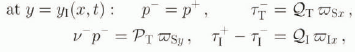
The boundary conditions used in this work are as follows: The free surface y = y_F(x, t) is assumed stress free, i.e.T_I n = 0, where n is the unit normal to the surface.

At the base y = y _Β(x, t), no-slip is assumed, i.e. υ _α = 0.

Since the upper layer contains no till, the interlace y = y _I(x, t) is material with respect to till, yielding the kinematic condition

(2.8)

where u _α , and υ _α represent the x and y components of υ _α . The mass and momentum-jump conditions are

(2.9)

where Equation (2.9)₁ was used to write Equation (2.9)₂, 〚Ψ〛 = Ψ ⁺ – Ψ ⁻ (+ for the upper, pure-ice layer, and – for the till–ice layer) and ϖ _α represents a constituent interaction force conceptually analogous to m as given in Equation (2.7), but one on the interface between the lower till–ice layer and the upper pure-ice layer, rather than in the bulk. In the till ease (α = T), the first term in Equation (2.9)₂ vanishes; as for ice, dimensional considerations show it to be negligible. Consequently, we have

(2.10)

In general, the sum of the constituent interface momentum-exchange terms is zero, i.e. ϖ _T + ϖ _I = 0, ensuring momentum balance in the mixture as a whole at the interface.

The presence of a non-zero constituent interface interaction force ϖ _α in Equation (2.10) can be motivated as follows. Consider a pillbox with its upper surface in the pure ice and its lower surface in till–ice mixture, with both of these surfaces parallel to the interface. Assume for simplicity a state at rest with no shear stresses. Surface forces from the pillbox sides can be ignored (or vanish in this simple case when the force balance in the direction of the pillbox thickness is considered, which we do here for the sake of simplicity). With the top as the + side, and the bottom as the – side, Equations (2.4) and (2.10) then imply

(2.11)

with ϖ _α = ϖ _α • n. Now, since p ⁻ = p ⁺ follows from Equation (2.11)₃, and p ⁺ ≠ 0, setting ϖ _α = 0 in Equation (2.11)₂ implies v ⁻ = 0, i.e. no jump of till volume fraction across the interface in this case. As such, for a given value of p ⁻ , Equation (2.11)₂ couples the “magnitude” of the jump in the till volume fraction (i.e. 〚v〛 = v ⁻ ) to that of the till–ice momentum-exchange interaction ϖ _α at the interface; in particular, the larger the till–ice momentum exchange at the interface, the larger the jump in till volume fraction. Consequently, ϖ _α clearly defines the sharpness of the interface between the till below and pure ice above, with ϖ _α = 0 corresponding to no interface (in the sense of a jump in the till volume fraction) at all. Observations (e.g. Engelhardt and others, 1978) indicate that indeed the interface between the pure ice above and the till below is rather abrupt, or sharp; in other words, till is concentrated in the basal layer. In any case, we would also expect ϖ _α ≠ 0 on physical grounds; indeed, the steep gradient in the till volume fraction from the bottom to the top of the pillbox induces mechanical interactions (forces) between the till and ice which in the limit as the pillbox thickness goes to zero become corresponding interface interactions which are non-zero in general.

3. Dimensional analysis and simplification

In this section; we adapt the above balance and constitutive relations to the two-dimensional, parallel-sided slab idealization of a glacier or ice sheet dealt with in this work (see Fig. 1). To this end, we work with the following scalings:

(3.1)

Here L, H, U, V and T represent a typical length, thickness of the two-layer system, x velocity, y velocity and time, respectively, chosen such that T = L/U = H/V.

Substituting Equations (3.1) into Equations (2.2)–(2.7), and introducing the thin-layer approximation ε = H/L ≪ 1, we obtain the following non-dimensionalized component forms of the model relations for the lower mixture layer:

(3.2)

to O(l) in ε, where now, and in the rest of this work, all variables are non-dimensional. The notation f _,y indicates a partial derivative of a quantity f with respect to y. In these last relations appear the non-dimensional quantites , , and ; furthermore g: = lgl; in addition, we have introduced τ _α = S _αxy (for more details, see Hutter and others, 1994). Similarly, the boundary conditions from Equations (2.8)–(2–10) become

(3.3)

(3.4)

(3.5)

with , and ‘ . The dimensionless equations in the upper layer are

(3.6)

from which we obtain

(3.7)

where y _F = 1 and the boundary conditions (3.2) were used. From Equations (3.5)₂, we infer that if the till volume fraction ν ⁻ does not vanish, the interface till–ice interaction force ϖ _Sy in the y direction must differ from zero. In the next section, these quantities are prescribed and their effect on the thickness and mechanical behaviour of the basal layer is quantitatively investigated in some simple cases.

4. Numerical solutions and discussion

The relations (3.2)_1,2 can be rewritten in the forms

(4.1)

representing two coupled equations in two unknowns v and p. In addition, restricting attention for simplicity to the case of constant viscosities, i.e. [G-entity] _α = constant, Equations (3.2)_3–6 can be combined to obtain the single relation

(4.2)

for u = u _T – u _I. If y _I is given, we can integrate the first two equations containing only v and p numerically with the boundary conditions (3.5)_1,3. From Equations (3.2)_5,6, (3.5)_2,4 and (3.7)₂, there follows u, _y ⁻ = 1 – y _I at the interface. The relation (4.2)₃ together with the boundary conditions u, _y ⁻ = 1 – y _I and u(yB) = 0 constitutes a two-point boundary-value problem, which can be solved numerically using a shooting technique. The shear stress τ _α is then obtained via numerical integration of Equations (3.2)_3,4 with Equations (3.5)_2,4 and the solutions of u and v. Finally, the velocity u _α is obtained by integrating Equations (3.2)_5,6 with Equation (3.4). It is reasonable to assume continuity of the ice velocity through the interface, i.e. u _I ⁻ = u _I ⁺ as the kinematical relation at the interface, which can be used to determine y _I via a predictor-corrector method. Giving an initial value for y _I , we calculate u _I ⁻, u _I ⁺ and compare them, If their difference is not sufficiently small, we correct y _I and repeat the computation until the difference |u _I ⁻ = u _I ⁺| becomes negligible.

For the numerical solutions, we chose H = 1000 m, [R] = 2.7, [G]_I = 1, [G]_T = 1, [M] = 1 and [P]_T = 1; the first of these is an appropriate order-of-magnitude value for the thickness of an ice sheet and the other values are chosen for simplicity. In particular, note that [G]_T/[G]_I = [R] μ _I/μ _T, so that these assumptions correspond to assuming that the viscosity of the “granular” till is about three times that of ice. Further, we assume that ϖ _Sx , ϖ _Ix and ϖ _Iy are negligible for simplicity and focus on ϖ _Sy , which is prescribed. Equation (3.5)₃ allows the till volume fraction v ⁻ at the interlace to be evaluated. Since v ≈ 0.85 at the base is the largest physically reasonable value (personal communication from G. Clarke), y _B = y(v = 0.85) is numerically determined in our computations.

As shown by Hutter and others (1994), one obtains only trivial solutions of Equations (4.1) when δ = 1, i.e. a single-layer, single-constituent “mixture.” Svendsen and others (1995) investigated the effects of varying δ for v ⁻ = 0 on the till volume fraction, pressure, shear stress and velocity profiles in a single-layer mixture model for a glacier or ice sheet. In particular, they showed that the most realistic till volume-fraction profiles arise for the case δ = 0.95. Here, we use this value of δ and vary v ⁻ , which is tantamount to varying ϖ _Sy in the context of Equation (3.4)₂, and it is easier to implement numerically. In particular, we look at the cases v ⁻ = 0.01, 0.1 and 0.5; the effects of this on the vertical profiles for till volume fraction, saturation pressure, ice velocity, till velocity, ice shear stress and till shear stress in the lower part of the two-layer system (0 < y < 0.1) are shown in figure 2a–f. The most significant aspect of these results is the upper extent of each curve, which marks the interface position in the two-layer system. Indeed, varying v ⁻ does not alter significantly the form of the profiles, i.e. the qualitative behaviour of the solution, nor even their quantitative values, but rather the lower till-layer thickness. Looking for example, at the till volume-fraction profiles in figure 2a, we see that, with increasing v ⁻ , i.e. an increasingly sharper interface, the lower till layer becomes thinner. Comparing this trend with interface values p ⁻ of p shown in figure 2b (upper lefthand values on each curve), which increases with v ⁻ , as well as with Equation (3.4)₂, implies that ϖ _Sy is also increasing with decreasing basal-layer thickness. Consequently, the stronger the till–ice interactions at the mixture-ice interface, the thinner and sharper the resulting basal layer. From the quantitative point of view, the effect of varying v ⁻ , and so ϖ _Sy , on the fields is most noticable in the case of the saturation pressure (Fig. 2b) and shear stresses (Fig. 2e and f); indeed, these increase with increasing basal-layer thickness (at a given depth in the layer) and so indirectly with increasing till–ice momentum exchange.

Fig. 2. Till volume fraction (a), saturation pressure (b), ice velocity (c), till velocity (d), ice shear stress (e) and till shear stress (f), profiles with depth (all dimensionless) for three values of ν⁻, i.e. ν⁻ = 0.01 (curves with squares), ν⁻ = 0.1 (curves with circles) and ν⁻ = 0.5 (curves with triangles). For these calculations, we chose H = 1000 m, [R] = 2.7, [G]_I = 1, [G]_T = 1, [G] = 1 and [P]_T = 1 (see text).

One of the main purposes of the current work is to investigate the effect of till–ice interaction processes, both in the bulk, as represented by m in Equation (2.7), as well as on the mixture–ice interface, as represented by ϖ α in Equation (2.10), on the “geometry” of the two-layer system and, in particular, on the distribution of till in this system. From an observational point of view, it is exactly this latter aspect, i.e. the distribution of till in the system, that is most well-known. As shown in this and previous work, the bulk and interface momentum interaction between till and ice has a dramatic influence on this distribution, as well as on the thickness of the basal layer. The next step is to extend these considerations towards a more detailed model of the rheology and dynamic behaviour of the basal layer itself, taking in particular ice–till (and perhaps more importantly, free-water–till) interactions into account.