Introduction

The Norske Øer Ice Barrier (NØIB) is a large expanse of landfast ice that develops over the northeast continental shelf of Greenland (known as Belgica Bank) at around 79^˚30^' N (Fig. 1). Previous studies have concentrated on the NØIB being the southern boundary of the Northeast Water (NEW) polynya (Reference Schneider and BudéusSchneider and Budéus, 1997). To the east the NØIB is bordered by drift ice moving southward on the East Greenland Current (EGC). Under the NØIB a system of channels up to 460m deep separates the very shallow Belgica Bank from the rest of the continental shelf (Reference Wadhams, Wilkinson and McPhailWadhams and others, 2006). Through these channels the Northeast Greenland Coastal Current (NEGCC) flows northward, and this is hypothesized as the main factor in creating the NEW polynya (Reference Schneider and BudéusSchneider and Budéus, 1995). the first observations of the NØIB were by Koch in 1938 (Reference KochKoch, 1945) and were followed by studies using the US National Oceanic and Atmospheric Administration (NOAA) Advanced Very High Resolution Radiometer (AVHRR) (Reference VinjeVinje, 1982; Reference Schneider and BudéusSchneider and Budéus, 1995) which determined that the NØIB had remained in place since at least before 1983 through to 1994. There are significant interannual variations in the size and extent of the NØIB, although a central area of perennial fast ice was identified extending in a tongue from between Nørsk Øer and Hovgaard Øer out to the area of Tobias Island (79^˚20^'38^" N, 15^˚48^'28^" W). the floating glaciers of the northeast Greenland region are embedded in the NØIB and it appears to prevent the calving of icebergs from these into the EGC (Reference Reeh, Thomsen, Higgins and WeidickReeh and others, 2001). the complete break-up of the NØIB used to be a rare event, estimated to occur about every 50 years (Reference HigginsHiggins, 1989, Reference Higgins1991). However, the NØIB disintegrated in summer 1997 and every summer between 2002 and 2005, releasing significant numbers of icebergs, before re-forming the following autumn. This study examines the formation of the NØIB during the season 2003/04 through data from multiple satellite sensors and examines how these sensors respond to the changing fast-ice surface conditions. Factors that lead to the formation of the NØIB are also discussed and the question raised about the susceptibility of this fast-ice barrier to changes in the climate.

Fig. 1. Map of Belgica Bank and the coast of northeast Greenland showing locations referred to in the text. IBCAO: International Bathymetric Chart of the Arctic Ocean.

Data Sources

Early studies used sporadic airborne surveys and cloud-free satellite images to determine the fast-ice extent and character of the NØIB (Reference VinjeVinje, 1982; Reference Schneider and BudéusSchneider and Budéus, 1995). the increased availability of high-resolution satellite data in the past decade, including all-weather synthetic aperture radar (SAR), has made it possible to study the evolution of the NØIB through the seasonal cycle. In summer 2003 the NØIB had disintegrated completely, with open water present all the way to the coast including up to the calving front of the Nioghalvfjerdsfjorden glacier. It subsequently re-formed, reaching a maximum extent in late 2003 before breaking up in summer 2004 where a residual fast-ice front remained in the gulf between Lambert Land, Norske Øer and Hovgaard Øer. During this season the European Space Agency (ESA) Envisat satellite started to make data available to scientific researchers. Envisat carries the Advanced SAR (ASAR) instrument. This is the first of the modern multimode and multipolarization SAR sensors and is capable of imaging both small, 56–100km wide, areas at approximately 30m resolution, and large, 400 km wide, areas at 150m resolution (ESA, http://envisat.esa.int./pub/ESA_DOC/ENVISAT/ASAR/asar.ProductHandbook.2_2.pdf).This enables both detailed examination of sea-ice rheology and mapping of larger regions, making it an ideal tool for ice-chart production. Also available was the first-generation SAR satellite, the Canadian RADARSAT-1, which has provided data for sea-ice mapping since 1995. Importantly, for mapping the NØIB area at 79^˚30^' N, SAR is capable of imaging during cloud cover and winter darkness. However, as SAR measures radar energy backscatter, what it mainly sees is the roughness of a surface (Reference Onstott and CarseyOnstott, 1992). This is fine when sea ice and water have distinctly different roughnesses, but causes problems in situations such as stormy weather that increase the backscatter from open water, or summer when melt ponding on the ice surface forms a water layer that hides the ice beneath. To supplement the SAR sensors, the optical Moderate Resolution Imaging Spectroradiometer (MODIS) sensors on NASA’s Terra Earth Observing System (EOS AM) and Aqua (EOS PM) satellites were used. These have been flying since 1999 and 2002 respectively and can provide visual and infrared imaging in 36 bands at up to 250m resolution over 2330km swaths (NASA, http://modis.gsfc.nasa/gov/about/specifications.php). However, as these are optical sensors, they can only be used during cloud-free periods.

Low-resolution sensors provide synoptic Arctic and Antarctic coverage of the changing sea-ice situation. As the NØIB forms over such a large area it is useful to compare the response of these to the ice cover during the season and to the high-resolution regional information coming from other satellite sensors. the workhorse of low-resolution sensors is the passive microwave radiometer. Variants of these have been mapping sea-ice extent since 1972 when the single-channel electrically scanning microwave radiometer (ESMR) was launched on the Nimbus-5 satellite, but it is the multichannel Scanning Multichannel Microwave Radiometer (SMMR) (Reference Parkinson, Comiso, Zwally, Cavalieri, Gloersen and CampbellParkinson and others, 1987), Special Sensor Microwave/Imager (SSM/I) (Reference Bjørgo, Johannessen and MilesBjørgo and others, 1997) and Advanced Microwave Scanning Radiometer – EOS (AMSR-E) that have provided the data used for the majority of climatological sea-ice studies (Reference Comiso and NishioComiso and Nishio, 2008). In addition, radar altimeter sensors promise to achieve the same coverage, but for sea-ice thickness. Unfortunately their use in the Arctic has been limited by the latitudinal restriction on the satellite orbit, but fortunately the NØIB is within the range covered by the Radar Altimeter 2 (RA-2) pulse-limited sensor, and on the Envisat satellite. This can provide coverage up to 81.5^˚N (ESA, http://envisat.esa.int/pub/ESA_DOC/ENVISAT/RA2-MWR/ra2-mwr.ProductHandbook.2_2.pdf). Radar altimeter sensors provide a measure of the sea-ice freeboard, the portion of the ice above sea level, by accurate timing of the echo from a radar pulse generated by the satellite. the immobile sea ice of the NØIB is an ideal test area for all satellite sensors as it reduces the problems with changing satellite and target geometries.

Ground truth for the satellite observations over the 2003/ 04 season is provided by a research cruise of the RRS James Clark Ross (JCR), which visited the area in August 2004, and a Danish Meteorological Institute automatic weather station (AWS) on Henrik Krøyer Holme island (80^˚39^' N, 13^˚43^' W; World Meteorological Organization ID: 04313). the JCR carried the Autosub autonomous underwater vehicle (AUV), a robot submarine equipped to perform oceanographic measurements under ice and to map the topography of the ice canopy using a Kongsberg EM2000 multibeam sonar. One Autosub mission, M365 on 21 August 2004, took the AUV from the NØIB fast-ice edge 67 km across Belgica Bank and into the Norske Trough (Reference Wadhams, Wilkinson and McPhailWadhams and others, 2006). Data on the background meteorology for the season are available from Henrik Krøyer Holme station. This is an AWS with air-temperature, humidity, pressure, and wind-speed-plus-direction sensors, and has been operating since 1985 (Reference CarstensenCarstensen and Jørgensen, 2009).

The NØIB in 2003/04

Mapping of the fast-ice edge was conducted by manual (human) analysis, as used to generate ice navigation charts by the Norwegian Ice Service, using images from Envisat ASAR and MODIS for 42 different dates (for 6 of these see Fig. 2). These were loaded into the Quantum Geographical Information System (GIS) and the fast-ice edge drawn by visual inspection of the images. Use of the GIS software allows vector polygon files of the fast ice to be generated and used for further automatic extraction of data values from the images or other spatial analysis. Accuracy of the fast-ice area values derived using this approach depends on the satellite data being used. Taking a 700 km long ice edge in the NØIB area and, at most, a two-pixel inaccuracy, the error range is ±140km² for Envisat ASAR and ±350km² for MODIS at 250m resolution.

Fig. 2. The NØIB at key dates in development: (a) 20 October 2003; (b) 16 November 2003; (c) 29 December 2003; (d) 23 April 2004; (e) 20 August 2004 (also showing the location of the Autosub M365 track and RA-2 analysis area); and (f) 5 September 2004.

For most of July and August 2003, there were only scattered drift floes and icebergs in the region. In September the drift ice returned and by 20 October 2003 there was some initial consolidation, of 22 600 km², in the fjords, Jøkelbugten and on Belgica Bank around Tobias Island and two large ice islands that had become grounded to the northeast (Fig. 2a and 6). Once the ice drift was restricted by these anchor points, the development of the NØIB was rapid.

Offshore fast-ice development took place over the shallow areas of Belgica Bank where a combination of grounded ridge keels and icebergs kept the drift ice in place. the fast ice in this area was a conglomeration of old ice from the EGC and new ice that formed in place acting as a glue. By 16 November 2003, 27 days later, most of the northeast Greenland coast was fast-ice fringed and the fast ice was starting to bridge the Norske Trough (Fig. 2b). the total fast-ice extent was 40 500 km². After this date the drift ice within the Norske Trough channel consolidated, resulting in an embayment in the fast ice extending up from the south for 120 km.

Further consolidation of the drift ice filled in the embayment and extended the fast ice out to ~60 km from the coast at Germania Land to the south by 21 December 2003. Where ice was formed in the embayment, in the lee of the existing NØIB fast ice, it was a near-perfect undeformed sheet. At the end of the year, the NØIB fast ice had reached its maximum extent of 103 600km² (29 December 2003; Fig. 2c), and formed an extensive fringe around the whole northeast Greenland coast. This configuration appears to be unstable, as the area reduced by about 18 500km² by 9 January 2004. Loss of fast ice occurred in the south of the area, below île-de-France (77^˚40^' N) and at the entrance to the Norske Trough, but it re-formed when quiet conditions allowed.

The NEW polynya started to open in March and by April was consistently open. In mid-April a 9000km² area of fast ice was lost at 79–80^˚N so that by 23 April 2004 (Fig. 2d) the NØIB fast ice had achieved a configuration at 68 300km² that remained remarkably stable for the following 3 months. This was in the form of an extension 105 km out from the Franske Øer and Norske Øer (south of Tobias Island and north of 78^˚13^' N). One reason for the stability of the fast ice may have been the presence of two large ice islands, around 5 km in length, grounded 41 and 65 km northeast of Tobias Island and which were protecting the seaward edge of the NØIB. For comparison, Tobias Island is 2.4km² in extent and these islands were each just over 10.5km². Once these became mobile on 29 July 2004, possibly after loss of fast ice around the NEW to the north, the break-up of the NØIB followed. We note that the protective effect of grounded ice islands and icebergs on the stability of fast ice was previously recorded by Reference VinjeVinje (1982).

On 29 July 2004 the fast ice of the NØIB was 53 300km² in extent. By 5 September 2004 this had been reduced to 12 700km². In the south this was due to loss of ice in the area of Dove Bugt and Store Bælt behind Store Koldewey island. A similar fast-ice bridge feature persisted between the south end of Store Koldewey and an unnamed offshore bank (75^˚52^' N, 16^˚39^' W) until September. on the day before the Autosub M365 mission (20 August 2004; Fig. 2e), the NØIB was 33 000km² in extent. Fast ice was lost through erosion of the northern and southern edges. the area identified as being a permanent ice tongue extending to Tobias Island in 1993 (Reference Schneider and BudéusSchneider and Budéus, 1997) was removed during the second half of August and beginning of September, although some ice remained fronting Nioghalvfjerdsfjorden. This left the core of the 2003/04 season NØIB bridging the Norske Trough to Tobias Island and the shallows of Belgica Bank, as it had on 23 April 2004, but with no fast ice to protect it to the north and south. the first part of September saw the ice bridge dismantled, leaving a remnant fast-ice island to the southeast of Tobias Island (5 September 2004; Fig. 2f). on the East Greenland coast a remnant fast-ice fringe remained, extending up from île-de-France and through the islands northward. Ice in Jøkelbugten and the fjords broke up and became mobile.

Analysis

The satellite data covering the NØIB were analysed both for temporal changes (Fig. 3) and spatial variations in the area of the Autosub M365 mission (Fig. 4). the fast-ice surface is modified by the annual cycle of freeze and melt, and by short-term meteorological events. This results in the satellite sensors seeing the ice differently through the season, with some sensors being more useful at certain times of the season than others.

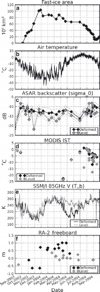
Fig. 3. Time series for the 2003/04 season showing: (a) the area of NØIB fast ice; (b) air temperatures from Henrik Krøyer Holme; (c) backscatter, σ ⁰, from Envisat ASAR; (d) MODIS ice surface temperature; (e) passive microwave (SSM/I) brightness temperatures; and (f) Envisat RA-2 freeboard. Where ‘level’ and ‘deformed’ lines are shown, these refer to the sea-ice conditions along the track of the Autosub M365 mission at 45–55km (for level ice) and 10–20 km (for deformed ice) from the fast-ice edge.

Fig. 4. Comparison of sea-ice thickness from Autosub mission M365 on 21 August 2004 as (a, b) level- and deformed-ice PDFs, (c) along-track profile, and (d–g) satellite data comprising (d) Envisat ASAR, (e) SSM/I, (f) MODIS and (g) Envisat RA-2 freeboard. Dates are yyyy-mm-dd. Distance is km into the NØIB from the fast-ice edge.

The meteorological data from Henrik Krøyer Holme station are the only long-term data on meteorology in the Belgica Bank area. Other measurements, from ships and buoys visiting the area, are sometimes available, but these are ephemeral and not from a fixed location. the average daily air temperature (Fig. 3) can be used to determine whether freezing and ice formation should be occurring in the vicinity. Likewise the wind speed and direction can indicate whether stresses are being applied to the fast ice that can lead to fracture. During the 2003/04 season, temperatures declined throughout the autumn of 2003, reached a minimum of –43.1^˚C on 24 January 2004 and did not approach levels where surface snowmelt could occur until a brief period around 19–24 April 2004. From mid-May, temperatures were either close to or above freezing, peaking at 6.8^˚C on 18 July 2004.

The weather was generally more turbulent during the equinoctial periods with gales (mean wind speeds >17.2ms^–1, Beaufort scale force 8). Autumn gale events occurred on 23 September 2003 and 5 September 2004, but were more frequent around the spring: 26 January, 19 February, 8 March, 26 March and 8 April 2004. the strongest of these was 19.6 ms^–1 on 20 February 2004. the final destruction of any remaining offshore fast ice from the previous season occurred during autumn. However, it was possible that drift-ice floes originating from the fast ice could survive in the region and be reincorporated into the next season’s NØIB. Gales during the spring reduced the area of fast ice that had grown during the autumn and winter. the period of greatest stability of the fast-ice edge coincided with the period of calmer spring and summer weather, from April through to the end of August 2004. During this period the highest wind speed was 12.1 ms^–1 (strong breeze, Beaufort scale force 6) on 24 June 2004.

The Autosub M365 mission on 21 August 2004 provided ice-draft statistical data which can be compared with the satellite information. Two sections along the track were selected for their dissimilar ice conditions: an area of deformed ice, made up of older floes conglomerated from the EGC, at 10–20km from the start of the mission, and an area of level ice, created in situ that season, at 45–55km from the start of the mission. A profile of the ice draft along the entire track and probability density functions (PDFs) are shown in Figure 4a–c. Summary statistics from the multi-beam sonar swath are shown in Table 1.

A total of 16 wide-swath medium (WSM), 20 image mode precision (IMP) and 1 alternating polarization precision (APP) scenes were acquired by the Envisat ASAR sensor between 24 June 2003 and 23 October 2004. These were processed to yield calibrated σ ⁰ backscatter values scaled in decibels (dB) and reprojected to a standard polar stereographic projection for the NØIB area (Fig. 1), using the Next ESA SAR Toolbox (NEST) software package. This also resampled the data to common grid spacings for the different imaging modes: 10 m for IMP and APP and 100 m for WSM. the images then had to be corrected for the different incidence angles, θ. WSM images cover most of the range of the ASAR sensor, from 19.2^˚ to 42.8^˚, with data covering the Autosub M365 track being from 28.2^˚ to 42.4^˚. the IMP images were all from image swath 2 (IS2) which ranges from 19.2^˚ to 26.7^˚. Because backscatter is strong at low incidence angles and decreases with increasing incidence angle, it was necessary to adjust data values to a standard incidence angle value, with the mid-range being 31^˚.

A large level area of ice was identified both in the satellite images and in the multibeam ice drafts from the Autosub M365 run between 37.1 and 57.2 km. This yielded dB degree^–1 slopes between pairs of IMP and WSM images, taken from the winter period, ranging from –0.035 to –0.239 (Table 2). For this study, an average value of –0.125 dB degree^–1 was used to adjust backscatter values to a standard incidence angle of 31^˚. This approximates reasonably well to this study (Fig. 5a), although further analysis is required on more extensive SAR datasets to see if it can be applied to Arctic sea ice in general. Comparison of before (Fig. 5b) and after (Fig. 5c) profiles for backscatter values along the Autosub track shows a general improvement.

Fig. 5. Correction of incidence angle for Envisat ASAR using data from the level NØIB fast ice. (a) Scatter plot of backscatter (σ ⁰) vs incidence angle for four pairs of WSM and IMP images (dates are yyyy/mm/dd). Black line shows the average –0.125 dB degree^–1 slope. (b, c) Profile plots of σ ⁰ along the Autosub M365 track where (b) non-adjusted and (c) adjusted for incidence angle. Black line is WSM 29 December 2003; grey line is IMP 9 January 2004.

Deformed ice has higher levels of backscatter, especially before the onset of melt in mid-April 2004 (Fig. 3c and 4d). By the time of the Autosub M365 mission, which had a near-coincident ASAR image at 12:37 UTC on 20 August, surface melt had reduced values for the deformed ice, creating homogeneous values across both types of ice, although there was very little difference between winter and summer values for level ice (Fig. 4d). This implies that the ice rheology as seen by SAR does partially correlate with the overall ice thickness, at least during winter and spring (Reference Comiso, Wadhams, Krabill, Swift, Crawford and TuckerComiso and others, 1991; Reference Hughes and WadhamsHughes and Wadhams, 2006).

The MODIS level 1B data and processing software, MODIS Reprojection Tool Swath (MRT Swath), was obtained from the NASA Level 1 and Atmosphere Archive and Distributed System (LAADS; http://ladsweb.nascom.nasa.gov/), at the Goddard Space Flight Center, Greenbelt, MD. This generated radiance values that were reprojected to the same area and projection as the Envisat data and standard grid spacing: 200 m for the 250 m, 400m for the 500 m, and 800m for the 1 km channels. For analysis the thermal channel values were converted to brightness temperatures, T _b, in kelvin, by the inversion of Planck’s equation (Reference Gumley, Hubanks and MasuokaGumley and others, 1994). Ice surface temperature (IST) was then estimated from MODIS channels 31 and 32, centred in the infrared at approximately 11.0 and 12.0 ^μm respectively (Reference Key, Collins, Fowler and StoneKey and others, 1997; Reference Riggs, Hall and AckermanRiggs and others, 1999).

Cloud filtering and visual quality control was performed to ensure that these values represented the ice surface (Reference Liu, Key, Frey, Ackerman and MenzelLiu and others, 2004). Using several of the thermal infrared channels, it is possible to determine whether the observation is of the sea or ice surface, or of some higher-level cloud. For this, channels 21 (3.9 μm), 28 (7.2 μm) and 31 (11.0 μm) were used.

There was a long period of the season (27 September 2003 to 11 April 2004) when no measurement of IST was possible due to cloud over the area of the Autosub M365 mission track. Elsewhere in the NØIB, however, there were sufficient clear areas, or areas veiled by thin cloud, to enable fast-ice edge mapping. Thermal channel data, particularly at 11.0 μm, clearly show any leads and were important for distinguishing the fast-ice edge. IST values show a good relationship to prevailing air temperatures (Fig. 3d). the high variability in this part of the NØIB region is due to the competing influences of winds blowing off the Greenland ice cap and the Greenland Sea. the results obtained along the Autosub track also indicate that this parameter may be able to indicate ice types, with lower temperatures occurring over level ice than over deformed ice (Fig. 4e).

Passive microwave SSM/I data from the US Defense Meteorological Satellite Program (DMSP) F-13 satellite were acquired from the NOAA Comprehensive Large Array-data Stewardship System (CLASS; http://www.class.ncdc.noaa.gov/). This takes the form of 3 hourly netCDF-format temperature data records which contain the antenna temperatures. These were converted to BT values using a first-order antenna pattern correction (APC) and coefficients for the F-13 SSM/I sensor (Reference Colton and PoeColton and Poe, 1999). the APC corrects for the incomplete radiometric coupling between the sensor reflector and feedhorn, cross-polarization coupling between channels, and side-lobe contamination. Changes in BT through the season indicate changing ice surface conditions, particularly snow cover, and meltwater ponding in summer (Fig. 3e). A rise in T _b in January appears to be related to the increasing proximity of the analysis region to the fast-ice edge and may be due to an ocean heating effect. Use of T _b values from all channels can also be used to determine the type of ice (Reference HughesHughes, 2009).

Level and deformed ice provide differing levels of emissivity that could be used for classification, particularly during the early periods of melt, some of which from the Henrik Krøyer Holme weather record appear to start occurring in mid-March, when level ice is still radiometrically brighter than deformed ice, particularly for the higher microwave frequencies (85 GHz) (Fig. 3e and 4f). This distinction disappears during mid-summer. the drawback with using the high-frequency channels is that these are affected more by atmospheric noise (Reference Lubin, Garrity, Ramseier and WhritnerLubin and others, 1997).

The final satellite sensor examined in this study was the Envisat RA-2. RA-2 data were acquired as geophysical data records (GDRs) from the ESA archive at Collecte, Localisation, Satellites (CLS), France, and processed to a format suitable for further analysis using the ESA Basic Radar Altimetry Toolbox (BRAT). the data covered cycles 17–31 (2 June 2003 to 8 November 2004) and BRAT was used to apply the atmospheric and geoid corrections contained within each GDR file. After processing in BRAT, the data for the study area, totalling almost 3×10⁶ points, were injected into a spatially enabled PostgreSQL + PostGIS database. This enabled further selection of data points within 10km of the track of Autosub mission M365. As the precise size of footprint of the RA-2 is not specified in the literature but is nominally 2–10 km in diameter (Reference Connor, Laxon, Ridout, Krabill and McAdooConnor and others, 2009), a safe buffer of 10km was placed around features that might affect the ice-freeboard results, such as land and the fast-ice boundary. This created a lozenge-shaped area of 1071km² with bites taken out of the southern edge, due to Tobias Island, and the northeast, due to the proximity of the fast-ice boundary (Fig. 1). Following this spatial filtering, the number of relevant data points was reduced to 7798.

Another parameter of the radar altimeter signal that can be used to filter out unwanted values is the pulse peakiness (PP) criterion (Reference Peacock and LaxonPeacock and Laxon, 2004). Values for PP are provided in the GDR data file; radar returns with a PP less than 3 (diffuse) can be classified as floes, and those with a PP greater than 30 (specular) as leads (Reference Connor, Laxon, Ridout, Krabill and McAdooConnor and others, 2009). Points with other values of PP are defined as unknown. Applying this criterion, the dataset was reduced to a possible 1934 points that should represent the freeboard values for fast ice, with 1907 as leads and 3957 as unknown.

A time series of daily average values for the test area, split between the areas of level and deformed ice, reveals no obvious patterns (Fig. 3f). Detection of points that the PP criterion delineates as ice was more likely in winter and spring, consistent with radar altimetry requiring the snow cover to be cold and dry (Reference Willatt, Giles, Laxon and WorbyWillatt and others, 2010). Apart from some anomalous values at the start of the season, the freeboard measurements for deformed ice are, as is to be expected, higher than those for level ice. There is a wider range of values for the deformed ice, consistent with the RA-2 taking profiles across different parts of the deformedice area. the level-ice values are more consistent because the area has few or no deformation features.

Examining the values obtained along the Autosub M365 track, apparently valid ice freeboard results were obtained for winter (dates around 12 April 2004) (Fig. 4g). the PP criterion also correctly identifies only ice, and no water or unknowns. In summer, when radar altimetry should be more unreliable due to surface melt, data from dates around 20 August 2004 show freeboard values in the level area for points that PP identifies as ice which appear to be consistent with the winter values, but also points identified as water or unknowns that appear to be valid measurements for deformed ice. In both winter and summer, some points are identified as ice yet have a negative freeboard. This appears to be due to errors in the atmospheric and ocean surface corrections supplied with the radar altimeter data files. Some of these are based on climate-model reanalysis data, which suggests that there is an inaccuracy of the model results in this region at these times. the use of fast-ice areas to assess the performance of radar altimetry including the use of PP as a filter for radar altimeter measurements will be the subject of further investigation.

Ice Islands

One feature of the NØIB observed in this study was how anchoring of the fast ice occurred on shallow water areas of Belgica Bank. This, and the bordering areas of drift ice, aided the fast ice in withstanding strong winds and accompanying swell, and would promote perennial retention of the NØIB if climate conditions deteriorated in favour of sea ice. However, the one large ridge observed by Autosub (33m deep; Reference Wadhams, Wilkinson and McPhailWadhams and others, 2006) would be unlikely to hold such an expanse of ice in place. Also observed at the time of the JCR cruise were large numbers of tabular icebergs with a freeboard of ~10 m, which implies a draft of around 80 m. These were up to 250m in length and quite capable of stopping some drift ice in the vicinity.

Because satellite images were downgraded for transmission in near-real time over limited bandwidth communications with the ship, it was not possible to access the full detail of satellite images at the time of the JCR cruise. Unbeknownst to the JCR, and discovered in this study, was the presence at that time of two large ice islands in the Belgica Bank area. These were tracked as they drifted at the beginning of the season to form the nucleus of the NØIB in October 2003 (Fig. 6a), and towards the end of the season as they broke out at the end of July, heralding the break-up of the NØIB (Fig. 6b). the northern ice island appears to have survived into the next season; the southern was lost to tracking after heading east off Belgica Bank and into the EGC. Both ice islands had a SAR signature distinct from that of the surrounding sea ice (Fig. 6c), and their drift tracks were also different to that of the surrounding EGC drift ice. the physical characteristics compared to the nearest land, Tobias Island, 41 km to the southwest, are shown in Table 3.

Fig. 6. Ice islands in the NØIB during the 2003/04 season. (a) Tracks into the NØIB during freeze-up, and (b) tracks out of the NØIB during break-up. Dates are yyyy-mm-dd. (c) Envisat ASAR IMP backscatter image of ice islands within the NØIB fast ice from 5 February 2004, 20:47:16 UTC. (d) One of many tabular icebergs encountered by JCR in August 2004 (photo by N.E. Hughes).

Although there are potential sources for ice islands in nearby Jøkelbugten and some of the glaciers of North Greenland (Reference HigginsHiggins, 1989), the ice islands found in 2004 are unusually large compared to the typical tabular icebergs found on Belgica Bank (Fig. 6d). Another possible origin is a break-out of the Ward Hunt Ice Shelf on Ellesmere Island, Canada, in 2002 (Reference Mueller, Vincent and JeffriesMueller and others, 2003). By the end of July 2004, just before the islands became mobile again, the northern island was exhibiting meltwater ponds, similar to a typical ice island, which ran parallel to its long axis. the southern island also exhibited a linear increase in SAR backscatter along its eastern side, which may have been the remains of one of the linear undulations. As these ice islands remained stationary in an area where the International Bathymetric Chart of the Arctic Ocean (IBCAO) marks about 50 m water depth, it can be assumed that they were grounded. Their presence during the initial formation of the NØIB in 2003/04 and the break-up of the northern part of the NØIB following their remobilization, suggests that the ice islands played a role in maintaining the NØIB, particularly during the long period between late April and the end of July when the fast edge was unaltered. an earlier study (Reference VinjeVinje, 1982) that identified an iceberg on Ob Bank as aiding fast-ice formation on Belgica Bank in 1981 appears to have been a misinterpretation of low-resolution infrared satellite imagery. Examination of the images shows that the ‘iceberg’ was the isthmus of fast ice extending down from Nordostrundingen.

Further tracking of the 2004 ice islands back to their points of origin, and forward to their break-up, will be the subject of a study using historical RADARSAT-1 satellite data.

Conclusion

The study demonstrated that a combination of high-resolution SAR and optical MODIS images is beneficial for mapping the fast-ice extent. As ice-drift products become more refined (T. Lavergne and S. Eastwood, http://www.osisaf.org/biblio/docs/ss2_pmseaicedrift_1_4.pdf), and with improved resolution (Reference Pedersen, Saldo, Lacoste and OuwehandPedersen and Saldo, 2005), these could also be incorporated into a processing routine that could first identify areas where fast ice may exist and use edge detection on the high-resolution images to map it. SAR backscatter, corrected for incidence angle and passive microwave emissivity, also shows variations due to ice rheology and, by proxy, thickness.

Alternatively, fast ice is also ideal for the calibration of satellite sensors. the principal problem with developing new algorithms to utilize new high-resolution SAR sensors is that sea ice is a moving target. This currently rules out any form of interferometry (InSAR) techniques, although new SAR constellation missions (e.g. Cosmo SkyMed, TerraSAR Tandem-X, and RADARSAT Constellation) may permit this. As fast ice is stationary, studies using it would allow such techniques to be tested.

Some of the most exciting new types of sensor that could radically improve our understanding of sea ice are those based on laser and radar altimetry. These offer the possibility of acquiring regular ice-freeboard information over wide areas which, if it could be incorporated into ice charting, could yield benefits to marine users in polar regions in terms of better trafficability (AMSA, 2009). Currently the assessment of the performance of these sensors is hindered by the inability to acquire coincident altimeter, high-resolution images, and ground truth data over areas of interest. Calibration studies over fast-ice areas would again remove critical differences in satellite and target geometry. In this study, a limited evaluation of the RA-2 on Envisat has shown some initial promising results for looking at ice freeboard in detail, as opposed to the temporal and spatially averaged climatological analyses normally presented. Further confirmation is also provided by the availability of under-ice upward-looking sonar data provided by the Autosub. This work will be continued with automatic processing of radar altimetry data using ice charts to provide polygon analysis areas which are expected to contain ice of the same type.

Since the 2003/04 season the NØIB has broken up in 2005 and in 2008. Although 2007 was the year of record minimum ice cover in the Arctic, this appears to have preserved the NØIB through until 2008 by sending a stream of drift ice south on the EGC. At the time of writing (summer 2010), the NØIB shows no signs of a break-up, and has a core area composed of 2 year old ice which has survived since the freeze-up in 2008.

The question remains as to whether the NØIB can act as an indicator of climate conditions. Certainly if the fast ice were to disappear and be replaced by EGC drift ice in winter, this would indicate a severe change in environmental conditions on the Belgica Bank area, with consequences for the coastal ecosystems of the area. Fortunately there appears to be little sign that this is likely to occur.