


INTRODUCTION
Jökulsárlón is an enclosed proglacial lagoon on the south-east coast of Iceland (Fig. 1). It borders Breiðamerkurjökull, which flows from the Vatnajökull ice cap and discharges ice into the lake at a rate of 260 ×106 m3 a−1 (Björnsson and others, Reference Björnsson, Pálsson and Gudmundsson2001), with calving front velocities of up to 5 m d−1 (Voytenko and others, Reference Voytenko2015a). The lake itself is connected to the North Atlantic Ocean through a channel ~70 m wide at its narrowest point and ~6 m deep. All tidal and residual flows to and from the lake are through this channel.

Fig. 1. (a) Aqua/MODIS satellite image of Iceland captured on 20 July 2008. The yellow box encloses Jökulsárlón lagoon. (b) False colour image of Jökulsárlón lagoon, Iceland. Breiðamerkurjökull is at the top left. Grounded small icebergs are obvious at the southern bottom of the image. The Breiðamerkurjökull ice face location is shown at various labelled dates.
Jökulsárlón formed in the 1930s as the glacier began to retreat. Since its formation the surface area of the lake has increased in size from ~5 km2 in 1960, to ~15 km2 in 1999 Björnsson and others (Reference Björnsson, Pálsson and Gudmundsson2001); its surface area in 2012 measured just over ~23 km2. The bed beneath Breiðamerkurjökull has a reverse slope such that the current configuration of the glacier is unstable and the lake is expected to continue to increase in area as the glacier continues its retreat (Björnsson and others, Reference Björnsson, Pálsson and Gudmundsson2001). Because of the shallow exit to the Atlantic Ocean, virtually all of the calving ice from Breiðamerkurjökull erodes within the lake and the meltwater is released within the lagoon. The effect of this meltwater flux is critical to the lagoon's hydrographic structure. Measurements in the 1970s showed that in winter Jökulsárlón was relatively fresh, and that its deepest regions (>100 m) had maximum salinities of ~12; in summer this dropped to ~4 as the entire lagoon was flushed by meltwater (Harris, Reference Harris1976). Harris (Reference Harris1976) also observed that saline water from the Atlantic Ocean was not able to enter the lake for the majority of the year and, when it did, the process was sporadic. We conclude that at this point in its history, the lake was relatively isolated from the ocean.
Between 1960 and 1982 the Breiðamerkurjökull ice front was fixed at a narrowing of Jökulsárlón just north of 64°03′N. This narrowing is labelled ‘pinch point’ in Figure 1b. Since the Harris (Reference Harris1976) study, the surface area of the lake has increased by a further ~15 km2, and a key driving force for the increase could be ocean/glacier interactions. Energy-balance studies of the lake (Björnsson and others, Reference Björnsson, Pálsson and Gudmundsson2001; Landl and others, Reference Landl, Björnsson and Kuhn2003) have demonstrated the importance of the heat from the ocean in the decay of the calved ice, and the Icelandic Road Authority has supported a project on the current ocean heat and salt budgets of the lagoon since 2011 (Ólafsson and others, Reference Ólafsson2013).
In this study, we investigate the hydrographic structure of the lake in late winter and the effect of the ocean on the calving ice front. We describe the dataset collected, present analyses of the tidal connection with the ocean and the hydrographic structure across the lagoon, and finally perform an analysis of the submarine melting at the ice face.
METHODS
We conducted four surveys from 20 to 22 April 2012, from a small boat to determine the early spring hydrographic structure of Jökulsárlón. Measurements were made using an internally recording YSI CASTAWAY CTD, which also recorded the GPS position before and after deployment so that drift could be monitored. At each station, the CTD was lowered to ~5 m depth for at least 2 min to allow the sensors to equilibrate, it was then raised to the surface and lowered in one continual movement to either the lagoon bed, or the maximum length of the line (~90 m). Data were downloaded at the end of each day. The boat was not equipped with an echosounder and we relied on University of Iceland maps for our station locations.
The lagoon and the location of the CTD measurements is shown in Figure 2. It was not possible to get within 1 km of the entrance of the lagoon because of grounded icebergs (as seen in Fig. 1b). Section 1 (13 stations, triangles) went from the centre of the glacier directly towards the entrance of the lagoon, and along the deepest channel noted in our charts. Section 2 (11 stations, inverted triangles) was across the ‘pinch’ point (Fig. 1b). Section 3 (10 stations, squares) was from the far western end of the Breiðamerkurjökull directly towards the sea channel, and section 4 (17 stations, diamonds) was along and within 2–30 m of the front of Breiðamerkurjökull. Finally, 8 CTD casts (Fig. 2) were taken in the narrow channel connecting the lagoon to the sea. Three of these were on the ebb tide and five on the flood tide.

Fig. 2. The lagoon CTD survey. Upward triangles are CTD locations on section 1, downward pointing triangles CTD locations on section 2, squares CTD locations on section 3, and diamonds as CTD Locations on section 4. Circled symbols mean the CTD reached the lagoon bed. Channel CTD stations are marked with a cross. Bathymetric data are from the University of Iceland. The downward triangle shaded red is station 17 and is discussed with reference to Figure 10.
Prior to our CTD survey, the University of Iceland placed four small sensors manufactured by Star-Oddi in the channel between Jökulsárlón and the North Atlantic Ocean: two of which measured pressure and temperature, and two which measured temperature and salinity. Both types sampled in synchrony every 10 min and were deployed on 12 July 2011, and recovered on 15 November 2011 (126 days in total).
RESULTS
Tidal flow into the Lagoon
Figure 3a shows the pressure record in the channel for the month of August 2011, Figure 3b shows the spectral analysis of the entire 126-day record and, Figure 3c shows the tidal prediction for the same time period in Figure 3a. Neap tides (8 and 23 August), were ~0.39 m and spring tides (3 and 15 August ~1.38 m. The median peak to peak tidal range was 0.95 m. We used the software package t_tide to spectrally analyse the 126 day pressure record (Pawlowicz and others, Reference Pawlowicz, Beardsley and Lentz2002): 21 significant tidal frequencies were identified and a tidal prediction based on these frequencies returned. Figure 3b shows the highest energies in the spectral signal that are the semi-diurnal components M 2 (the principal lunar component) and S 2 (the principal solar component). There are also sharply defined peaks in the diurnal K 1 (luni-solar component) and O 1 (principal lunar component) frequencies. There are broader peaks at frequencies above 2 cycles per day, particularly at the harmonic tidal constituents M 4 and M 6 and then smaller-amplitude, broader peaks close to 5 and 7 cycles per day, and at the M 8 frequency. These higher frequencies are generally observed in shallow waters and result from the interaction of the lower frequency tides with local topography. Their impact can be seen in the tidal prediction shown in Figure 3c, and the superposition of different frequencies means that successive tidal peaks (marked with a circle) do not uniformly rise and fall with the spring-neap cycle. The dashed line above the prediction shows the peak to peak tidal range. In the period from neap to spring tidal maximum (e.g. from 8 to 15 August) successive peaks show large differences in maximum tidal height. This difference is not observed from the spring maximum to the neap tidal minimum (15–20 August). Such asymmetry between the neap-spring and the spring-neap range is observed throughout the entire 126 day record.

Fig. 3. Data and predictions from one Star-Oddi sensor in the channel to the North Atlantic. (a) The pressure record for August 2011. (b) The spectral energy of the tides from 126 days of data. (c) The solid line is the tidal prediction for August 2011, circles on this line are successive high and low tides. The dashed line is the daily tidal range.
Figure 4 shows the temperature and salinity recorded in the channel over a 24 h period on 1 August: the period of tidal inflow into the lagoon is highlighted in grey. At ebb and low tides the temperature is ~2.4°C, and during the relatively short flood, the temperature jumps up to ~9.4°C in just 20–30 min (an increase of ~7°C). The corresponding salinity change is from ~11.2 at ebb and low tides, to ~32.8 during flood tides (an increase of ~21.6). We term this warm saline water Coastal Atlantic Water (cAW) as it is Atlantic Water that has been modified close to the coast by terrestrial runoff from Iceland. Figure 3a shows that this observation is close to the spring tide (1 August) and we expect the tidal range to be close to the maximum (Fig. 3c). The difference between successive high tides is shown in Figure 4 as a difference in duration that cAW is observed: in the first high tide at 0520, the pulse duration is ~1 h 50 min, whereas at 1700 the pulse is ~2 h 50 min.
Fig. 4. The Temperature and salinity recorded in the channel between the lagoon and the North Atlantic Ocean for the 1 August 2011. Grey regions are when the flow is into the lagoon.
These consistently occurring pulses of warm, salty cAW have a density of ~1026 kg m−3. Taken together Figures 3, 4 demonstrate that unlike presented in Harris (Reference Harris1976), there is now a strong inflow of cAW into the lagoon with the tidal cycle. The strength of this tidal inflow was recorded using a SonTek Argonaut acoustic Doppler current Profiler on 22 April 2012. Over two short measurement cycles on the flood tide the inflow into the lagoon was measured at 425 m3 s−1. This is higher than the average tidal flow of 200 m3 s−1 measured over a 2 h period presented in Björnsson and others (Reference Björnsson, Pálsson and Gudmundsson2001), but peak values of 750 m3 s−1 have been recorded (Björnsson, Reference Björnsson1996) and given the duration of the tidal pulses shown in Figure 4 and the observed lake tidal range 0.2 m (Zóphóníasson and Freysteinsdóttir, Reference Zóphóníasson and Freysteinsdóttir1999), they are consistent. A typical flood tide of duration ~2 h 10 min equates to 3.3 ×10⁶ m3 of warm saline cAW water flowing into the lagoon each tide.
This inflowing water has a density anomaly of 8–14 kg m−3 over the lagoon waters, implying it descends rapidly as a dense plume. It was not possible to sample the plume because of grounded icebergs in the lagoon entrance (Fig. 1b). While the slope into the lagoon is relatively gentle at ~3.5°, the high temperature and salinity signal of the tidal inflow will rapidly descend this slope and mix with ambient lagoon waters through entrainment (Baines, Reference Baines2001).
Hydrographic sections across the lagoon
Next, we show three of the four hydrographic surveys across the lagoon to discuss the hydrographic state. Data from section 2 across the ‘pinch point’ (downward triangles) is not presented as a section as it does not add to the argument presented; however, the data are used in the temperature and salinity analysis below. The warm salty inflow of cAW observed in Figure 4 is absent in all sections
Section 1
In Figure 5 only the two stations closest to the lagoon entrance sampled the full water column, and the densest water here had a temperature of ~1.83°C, salinity ~20.82 and a potential density anomaly of 16.6 kg m−3, considerably lower than observed in Figure 4. We conclude that the cAW that enters the lagoon is either diluted very close to the channel entrance, or does it not reach the deeper waters along this path. The temperature plot (Fig. 5a) shows at the surface the three stations closest to the channel entrance are cold and below 0.75°C. Figure 5b shows this colder surface water is the freshest sampled on this section and, since this water is not entering the lagoon (Fig. 4), it is a result of the melting of the small locally trapped icebergs (Fig. 1b). At 30–40 m depth both the isotherms and isohalines are approximately horizontal. Above this depth with the exception three stations closest to the ice face isotherms and isohalines slope upwards from the lagoon entrance towards the ice face. The cold layer in the 10–20 m depth range is the remnant of the water cooled during winter. Beneath ~40 m depth both isotherms and isohalines generally descend from the lagoon entrance to the ice face. The most saline water observed (20.83) is at the ice face and at the maximum depth recorded.

Fig. 5. The hydrographic data recorded along section 1 on 20 April 2012 from the centre of the face of Breiðamerkurjökull towards the narrow channel (Fig. 2, upward triangles). Grey triangles are the locations of the CTD stations, circles indicate the station sampled to the lagoon bed. (a) Temperature (°C), (b) Salinity.
Section 3
Temperature and salinity profiles collected on section 3 (Fig. 6) ran from the western edge of Breiðamerkurjökull and close to the only visible source of turbid meltwater outflow, out to the grounded icebergs at the lagoon entrance (Figs 1b, 2). As with section 1 (Fig. 5), there is a divergence in slope of the isotherms and isohalines either side of a depth of ~30–40 m at a temperature of ~1.25°C, and a salinity of ~19.5. Above this depth, the coldest temperatures were at ~15 m depth (~0.5°C) and observed at the two stations closest to the ice face, and there is again a general freshening of waters towards the lagoon entrance. Below ~40 m once more both the isotherms and isohalines slope down into the lagoon. The most saline water (>22) sampled section within the lagoon was close to its channel inflow at 80 m depth (4.4–5.2 km), and a salinity increase is observed in the water at the deepest depth adjacent to the ice face.
Section 4
The hydrographic section along the Breiðamerkurjökull face is in Figure 7. The stations were <30 m from the ice face at the centre, and virtually adjacent to the ice at the east and west extremities. Figure 2 shows that most of the CTD stations along the ice face reached the lagoon bed – the exception being the over the central stations at 0.8–2.4 km. In contrast to Figures 5, 6, there is extensive vertical temperature structure that is not readily apparent in the salinity and density sections because the strong vertical temperature gradients are compensated by salinity variations. From the surface down to ~5 m depth, the temperature reveals a warm layer between 1.4 and 2.2 km that is warmest in the centre of the face that is discussed below. Beneath this warm surface is the cold layer observed in sections 1 and 3 (Figs 5, 6) and below 50 m depth (0.6–2.8 km) there is a complicated vertical temperature structure: warm and cold layers interleave and there are sharp temperature gradients of up to 1.5°C over 7 m in the vertical. As discussed below, there is evidence that the water is not statically stable in some locations. The salinity and potential density sections in Figure 7 show that across the ice face both isohalines and isopycnals are generally horizontal except at the boundaries where the CTD reached the lagoon bed. The most saline (and so dense water) observed in the section was between 0.9 and 1.7 km and below 80 m depth, and in the range 21–22 >17 kg m−3), much fresher than the observations in the channel.
Surface heating close to the ice face
The warm water observed at 0–6 m depth in section 4 (Fig. 7a) was not observed in the other sections. Figure 8 shows the temperature data recorded within the lagoon and maps at three depths chosen to reveal the general character. Figures 8a, b show that the largest range of temperature within the lagoon occur at 1.5 m depth. The warmest water at this depth was adjacent to the ice face and generally, there is cooling with distance from Breiðamerkurjökull with the coldest temperatures close to the lagoon entrance. Figures 8a, c show that by 9 m depth the range of temperature across the lagoon is at a minimum and the signal of the warm water observed close to the ice face is absent. The final selected depth at 72 m (Figs 8a, d) shows the location of the deepest stations in the lagoon; there is a larger temperature range than at 9 m depth and at this depth in contrast to the near surface the water cools towards the ice face.
Combined with the sections of Figures 5–7, Figure 8 shows that there is a cooler, fresher and lower density pool of water south of the 1982 ‘pinch point’ due to the local melting of trapped calved glacial ice at the southern end of the lagoon. Below ~50 m depth because the isohalines (and isopycnals) are sloping down towards the ice (Figs 5, 6), the deeper water is warmer in the direction of the ice front- although coldest at the actual Breiðamerkurjökull face.

Fig. 6. The hydrographic data recorded along section 3 on 21 April 2012 from the west end of the Breiðamerkurjökull face to the narrow channel (Fig. 2, squares). Grey triangles are the locations of the CTD stations, circles indicate the station sampled to the lagoon bed. (a) Temperature (°C), (b) Salinity.

Fig. 7. The hydrographic data recorded along section 4 on 22 April 2012 along the face of Breiðamerkurjökull (Fig. 2, diamonds). Grey triangles are the locations of the CTD stations, circles indicate the station sampled to the lagoon bed and the red triangle marks the location of CTD station 51 as discussed in Figure 11b. (a) Temperature (°C), (b) Salinity. (c) the potential density anomaly (kg m−3).

Fig. 8. (a) Vertical profiles of the temperature of all CTD stations recorded in the Lagoon. The three levels marked in dashed black are shown in subsequent subplots. (b) The lagoon temperature at 1.5 m depth. (c) The lagoon temperature at 9.5 m depth. (d) The lagoon temperature at 72 m depth. Open circles indicate the depth level is below the depth of the lagoon bed.
Surface waters adjacent to the ice warmed over the data collection period and section 4 (day 3) was on average 0.8°C warmer than section 1 (day 1). Figure 7 shows the warmest water is concentrated in the upper 5 m of the ice face and warmest in the centre. The two sections extending from the ice face towards the entrance channel show the warmer signal extends only ~300 m from the ice.
One possibility for this observation could be solar heating of a wider near surface layer with local winds then shoaling the warmer water in a triangular wedge against the ice face. Taking the dimensions of the triangular wedge as 5 m thick, 3500 m wide and extending 300 m into the lagoon, the amount of energy to raise this volume of water by 0.8°C (T excess) is given by (volume × c p × T excess), where c p is the specific heat capacity of the water 4100 J kg−1 K−1, which is ~8.7×10¹² J. Given that 21 and 22 April 2012 had a patchy cloud cover with a typical insolation of 200 W m−2, the observed energy excess could be received by a 3×1 km surface area of water in ~7 h before then being shoaled against the ice by local winds with the warmest temperatures in the face centre (Figs 7, 8b). This excess heat is also responsible for a slight freshening and density decrease at the surface close to the ice face.
The temperature and salinity structure of the lagoon data
Figure 9 shows the potential temperature salinity relationship (θ − S) for the dataset collected within the lagoon. CTD measurements shown in Figure 9 are solid blue lines. The red square is the mean potential temperature and salinity of the lagoon inflow recorded in the channel during a flood tide, and the red circle the data at the same location during an ebb tide. These two symbols represent the conditions of the tidal flood and ebb in in April 2012 (see for example Fig. 4). The θ − S relation of the CTD data >10 m depth generally lies along the mixing line between the two extremes presented by the inflow and outflow (black dashed line in Fig. 9). The scatter around this mixing line is due to input from two sources: ice melt (both from the glacier face and icebergs) and freshwater runoff from the glacier (from surface melt and subglacial discharge). This variation about the mixing line, along with the red and green dashed lines is discussed below. Above 10 m depth Figures 5–8 show that the warming and associated surface freshening is south of the 1982 pinch point. The least dense cold water we observed was close to the lagoon entrance.
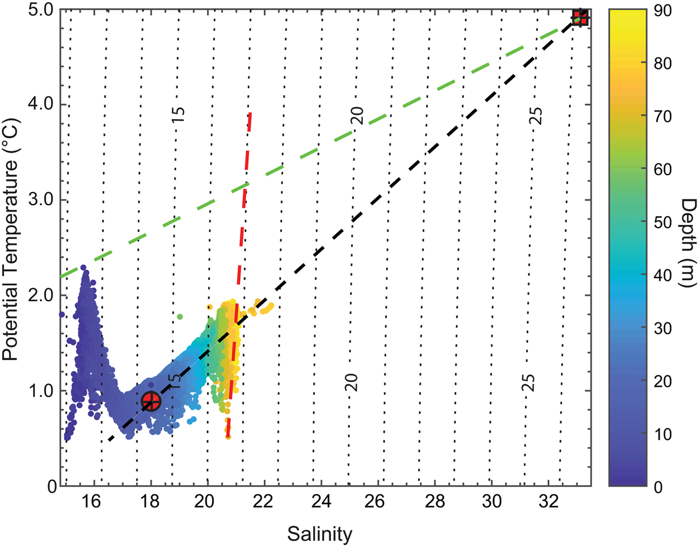
Fig. 9. The θ − S plot for the CTD data collected in Jökulsárlón lagoon 20–22 April 2012. The red square is the mean inflow water, the circle is the mean outflowing water, the black dashed line a mixing line between these. The red dashed line is a Gade Melt line described in the text (Eqn (4)) and the green line a mixing line between freshwater runoff from the glacier (SgFW θ = 0°C, S = 0). Density anomaly curves are shown as dotted lines labelled at 5 kg m−3 intervals.
Within the lagoon there is a periodic inflow of heat and salt close to the bed due to tidal effects (square in Fig. 9 and grey shading in Fig. 4), while heat is being absorbed and salinity reduced through ice melt and freshwater input resulting in water leaving the lagoon with properties close to the circle in Figure 9 (unshaded regions in Fig. 4). Figure 10a shows the vertical profiles of all of the CTD data and it reveals that away from the ice face the range of temperature and salinity and density anomaly are relatively small. Highlighted in red in both Figures 9, 10 is the profile from CTD station 17 (location shown in Fig. 2), which was recorded at the eastern end of section 2 and did not reach the lagoon bed. Beneath 14 m depth this station lays on the direct mixing line between the waters flowing in (square in Fig. 9) and exiting (circle in Fig. 9) the lagoon, and because it is both full depth and away from the direct influence of Breiðamerkurjökull, we consider it reflects effectively the background state of the lagoon.

Fig. 10. (a) Vertical profiles of temperature, salinity and potential density. In red line Station 17 (recorded on section 2 and highlighted in Fig. 2). (b) The θ and S data from Station 17 (black stars), red dashed is the advection/diffusion modelled temperature and salinity(red dashed line).
DISCUSSION
Advection and diffusion
Because beneath 14 m depth, station 17 lies virtually on the black dashed mixing line in Figure 9 we can consider this as an advection/diffusion problem, where the constantly renewed deep water properties and the near surface properties are a balance between vertical upwelling and diffusion from the deep water. Such a straightforward situation is described in Craig (Reference Craig1969), and a solution presented in Glover and others (Reference Glover, Jenkins and Doney2011) is described in Eqn (1),
 $$k_{\rm z} \displaystyle{{\partial ^2 C} \over {\partial z^2}} = w\displaystyle{{\partial C} \over {\partial z}}$$
where k z is the vertical diffusion, z the vertical co-ordinate, C a conservative tracer, which in this case is potential temperature θ or salinity S, and w the vertical velocity. The solution to (1) is given by,
 $$C = a_1 + a_2 e^{z/z{^\ast}} $$
where a 1 and a 2 are constants of integration determined by the boundary conditions. z* is a scale height giving the relative importance of mixing and advection and is given by,
 $$z{^\ast} = \displaystyle{{k_{\rm z}} \over w}$$
Solving for both salinity and temperature gives the scale height z* = 38.7 ± 1.6 m, and Figure 10b shows the temperature and salinity values of station 17 with the modelled vertical profiles as dashed red lines. This good fit demonstrates that the overall properties of the mid depth waters between 14 and 85 m depth are a product of advection and diffusion between the warm, saline oceanic waters flooding into the lagoon with the tide, and the surface waters resulting from the ice melt and freshwater input.
Typical open ocean values of k z are ~10−5 m2 s−1, but within an enclosed lagoon such as Jökulsárlón we can expect it to be higher, and so use 10−4 m2 s−1. Substituting this into Eqn (3) gives a vertical velocity w of ~0.2 m d−1 of upwelling (or ~80 m a−1), and it is this upwelling that determines the mid-depth lagoon temperature and salinity properties shown as the black dashed line in Figure 9. The advection/diffusion balance is relatively slow and because this is controlling the general properties within the lagoon beneath ~14 m, transient processes such as surface meteorological effects are not significant.
However, the properties of the lagoon waters within the advective/diffusion region are also modified by Breiðamerkurjökull in two ways: ice melt from the glacier face and icebergs, and subglacial freshwater discharge. Each of these sources alter the potential temperature salinity characteristics of the lagoon in different ways (Mortensen and others, Reference Mortensen2013).
Subglacial water and meltwater
Subglacial discharge will be sediment laden, have salinity 0 and temperature at the pressure determined freezing point T f. This will be just below 0°C in this lagoon. We term this buoyant water SgFW after the formulation presented by Mortensen and others (Reference Mortensen2013). When SgFW emerges the glacial environment due to its comparative buoyancy it ascends and mixes turbulently with the ambient water (Motyka and others, Reference Motyka, Hunter, Echelmeyer and Connor2003; Jenkins, Reference Jenkins2011; Motyka and others, Reference Motyka, Dryer, Amundson, Truffer and Fahnestock2013; Carroll and others, Reference Carroll2015). The SgFW includes near surface runoff. Recent work in the lagoon has suggested that the SgFW can emerge from the ice face in pulses (Voytenko and others, Reference Voytenko2015b), and this can be tracked from the ice face across the lagoon through the sediment plumes observed in satellite imagery (Hodgkins and others, Reference Hodgkins, Bryant, Darlington and Brandon2016).
The melting of ice modifies warm saline lagoon waters by release of latent heat and dilution. Gade (Reference Gade1979) was the first to derive an equation for the gradient of a line in θ/S space that would result from these processes, and a recent derivation was presented in Mortensen and others (Reference Mortensen2013),
 $$\displaystyle{{\partial T} \over {\partial S}} = \displaystyle{1 \over S}\left( {\displaystyle{L \over {c_{\rm p}}} - \displaystyle{{c_{\rm i}} \over {c_{\rm p}}} (T_{\rm i} - T_{\rm f} ) - (T_{\rm f} - T)} \right)$$
Here T and S are the temperature and salinity of the ambient sea water. The specific heat capacity of the sea water c p and the freezing temperature T f are calculated from the observed T, S and pressure, L is the latent heat of fusion (3.34×10⁵ J kg−1), T i the temperature of the ice (set at 0°C) and c i is the specific heat capacity of ice (2.1×10³ J kg−1 K−1). Lines in θ/S space with a gradient given by (4) are often referred to as Gade Melt lines (Gade, Reference Gade1979).
The potential temperature salinity plot shown in Figure 9 has a mixing line between the SgFW and inflowing water measured in the lagoon entrance (green dashed), a mixing line between the inflow and outflow measured in the lagoon entrance (black dashed) and a representative Gade Melt Line given by (4) (red dashed). While the general characteristics of the lagoon waters are set by a balance between advection and diffusion, deviations from the black dashed mixing line between the near surface and deep waters can be seen to be generally orientated along the gradient of lines given by Eqn (4).
Figure 11a shows an enlarged θ/S plot of the CTD stations on section 4 (Fig. 7). Using the three mixing lines we can describe the water properties at the ice face. At the surface with the previously noted warm surface layer down to 9 m the waters almost reach a mixing line between SgFW and the inflow to the lagoon (green dashed line). From here to the maximum measurement depth profiles broadly follow the black dashed line created by the advection/diffusion balance. Superimposed on this are repeated departures that are generally orientated with the gradient of Gade Melt lines. Figure 11b shows the θ/S profile for station 51 that was taken within 30 m of Breiðamerkurjökull (marked as a red triangle in Fig. 7). At depths >9 m this station has both the coldest and the warmest waters a depth on section 4. The relatively warm layer in Figure 7 from ~52–68 m and above 1.5°C falls directly on Gade Melt line 1, and the second very cold water region at ~72 m and the water beneath is along Gade Melt line 2. While it is difficult to sample for most tidewater glaciers, it is clear in Figure 7 that submarine meltwater is along most of the ice front. However, Figures 5, 6 show that relatively extreme characteristics of the water leaving the ice front are rapidly mixed with distance from the ice face.

Fig. 11. (a) The θ − S plot for the CTD data collected along the ice front of Breiðamerkurjökull on section 4. The black dashed line is a mixing line between the inflow and outflow to the lagoon. The red dashed line is a Gade Melt line described in the text, and the green line a mixing line between freshwater runoff from the glacier (SgFW θ = 0°C, S = 0). Density anomaly curves are shown as dotted lines labelled at 1 kg m−3 intervals. (b) The θ − S plot for CTD Station 51 on section 4 (location highlighted in red in Figs 7, 12).
Using a model based on salt and heat conservation and the observed temperature and salinity properties presented by Mortensen and others (Reference Mortensen2013), one can derive the percentages of fresh water and glacial melt present in the observed hydrographic sections. Because the direct melt signature is only observed along the Breiðamerkurjökull face, we restrict our analysis to section 4 (Fig. 7). Rather than repeat the derivation of Mortensen and others (Reference Mortensen2013), we present the key equations from their model. They are:
 $$f_{{\rm FW}} + f_{{\rm WT}} = 1$$
and
 $$f_{{\rm FW}} = f_{\rm i} + f_{{\rm SgFW}} $$
where f FW is the total fraction of fresh water in the sample, and f WT is the fraction of ambient seawater from the tidal inflow to the lagoon. This latter is given by f WT = Sobs/S WT, and S obs is the sample salinity and S WT the salinity of the inflowing water. The properties of the inflowing water are shown as the red square in Figure 9 with T WT = 4.9°C and S WT = 33.9. f FW is the sum of fresh water due to submarine melt (f i) and the subglacial discharge (SgFW). f SgFW can be determined from the intersection of the Gade Melt line at the sample temperature and salinities given by Eqn (4), and the mixing line between the SgFW and the temperature and salinity properties of the inflowing water – i.e. the green dashed line in Figures 9, 11. The final fraction f i is the glacial ice melt. From Eqns (4)–(6), the relative fractional contributions of the subglacial freshwater runoff (Fig. 12a), the fractional contribution of the water inflow to the lagoon (Fig. 12b) and the fractional contributions of the glacier ice melt (Fig. 12c) can be determined.

Fig. 12. The hydrographic data recorded along section 4 on 22 April 2012 along Breiðamerkurjökull ice face (Fig. 2). Grey triangles are the locations of the CTD stations, circles indicate the station sampled to the lagoon bed. The red triangle marks the location of CTD station 51. (a) The percentage fractional contributions of the subglacial freshwater runoff f SgFW, (b) the percentage fractional contribution of the ambient water inflow to the lagoon f SgFW and (c) the percentage fractional contributions of the glacier ice melt f i.
Figure 12 shows that the water structure is dominated – as would be expected – by the background advective/diffusive balance. Above 40 m depth the dominant factor is f SgFW, the subglacial discharge (12a). In the top 5 m more than 50% of the observed salinity distribution is a result of subglacial meltwater – most of this likely at near surface injection sites, and virtually all of the remainder being from the inflowing Atlantic water. Below 10 m depth the salinity distribution is principally determined by the salinity of the inflowing water, and the proportion increases up to the maximum depths; correspondingly there is a decrease in subglacial meltwater. Below 40 m depth the f WT makes up more >60% of the observed salinity, and this is due to the inflowing cAW and the advective/diffusive balance as discussed above. While the contribution of melting ice is not significant in these late winter measurements to the overall salinity distribution, it is significant in certain key regions.
Figure 12c shows the horizontal section of the fraction of the salinity distribution due to ice melt; it can be broken down vertically into two clear regions: above 9 m depth the proportion of the glacial ice melt is below 1%, and in the warmest surface waters encountered in the lagoon (Figs 7a, 8b) there are values close to 0% glacial ice melt. Although the scale of Figure 12a does not show it, there is an increase in the upper 9 m of f SgFW of 2%, but this does not coincide with the warmest waters in Figures 7a, 8b. This supports that the assertion near surface warmer water is from relatively recent solar heating coupled to a meteorological driver for the concentration of the water in the centre of the face.
Below ~9 m depth, Figure 12c shows that the glacial ice melt f i is generally above 1%; there is clearly structure in both intensity and distribution of the glacial ice melt signal, with discrete maxima. This structure is particularly notable below 50 m depth and there are three peaks of intensity in the f i signal (x = 1.1 km and ~62 m depth, ~1.7 km and ~72 m depth and ~2.5 km and ~55 m depth) where the values are close or above 2%. These peaks indicate multiple injection points of submarine meltwater leaving the ice face where it then entrains ambient water and its properties are moderated such that they are not detectable in the other recorded sections (Figs 5, 6). The three regions of increased f i reach different depths and without making unjustified assumptions about the original melt injection we cannot infer an entrainment rate.
There is a band of glacial ice melt f i <1% centred at ~60 m depth in the region 1.5–2.4 km. This lower value band shows that along the ice face the water is dynamic and the high melt value regions beneath are reaching neutral buoyancy at depth. Between 10 and 40 m depth there is again increased ice melt leaving the ice face, although at lower intensity than observed at greater depths.
SUMMARY AND CONCLUSIONS
Using hydrographic data from the Jökulsárlón lagoon and very close to the Breiðamerkurjökull face we have shown that in contrast with historical work (Harris, Reference Harris1976) the lagoon is now oceanic in nature, with a strong tidal inflow. This saline water has a density excess of 8–14 kg m−3 over the water leaving the lagoon and as a result the inflowing water rapidly sinks to depth. Overall, our results suggest that the salinity of the deep waters has increased from 4 to >21 since 1976. Once in the lagoon the saline water is, through an advective/diffusive balance, responsible for determining the temperature and salinity of the lagoon waters beneath the immediate surface waters down to ~90 m. Given such a balance takes time to be formed and this suggests, our early spring synoptic data are representative of longer term conditions.
The pathway of the Atlantic-derived water through the lagoon is clear. The most saline waters at depth are found adjacent to the ice face, which implies that after descending rapidly at the entrance to the lagoon, the saline water reaches the ice face along a deep trough >90 m depth (Björnsson and others, Reference Björnsson, Pálsson and Gudmundsson2001; Landl and others, Reference Landl, Björnsson and Kuhn2003). At the ice face, there is, compared with the other hydrographic sections across the lagoon, a complex hydrographic structure with multiple interleaved warm and cold regions, indicating subglacial discharge from the glacier and submarine melt. This should not be surprising given visual evidence of high permeability above the water level and deep crevassing north of the ice face (Mottram and Benn, Reference Mottram and Benn2009) and relatively fast ice velocities at the ice front (Voytenko and others, Reference Voytenko2015a). The heat salt balance model of Mortensen and others (Reference Mortensen2013) shows the hydrographic structure at the ice face in the advective/diffusive region below ~14 m depth is the result of a complex pattern of inflowing cAW, subglacial discharge and submarine melt. Multiple injection points of meltwater are observed but the signals of these have already been mixed and diluted within 1–200 m of the ice face. This mixing would be enhanced by subglacial discharge plumes emerging from the ice face in discrete pulses (Voytenko and others, Reference Voytenko2015b).
There have been two published studies of the melt of Breiðamerkurjökull into Jökulsárlón lagoon (Björnsson and others, Reference Björnsson, Pálsson and Gudmundsson2001; Landl and others, Reference Landl, Björnsson and Kuhn2003), and both used the best hydrographic data then available – from 1974 (Harris, Reference Harris1976). Landl and others (Reference Landl, Björnsson and Kuhn2003) estimated that 60% of the heat that melts the ice in the lagoon comes from the ocean, and they gave a range of heat into the lagoon as being 882–2940 MW a−1. They noted that this was the largest term in their melt calculation. With the changes observed in the size and hydrographic structure of the lagoon from 1974 to 2012, approximately seven times more heat is entering Jökulsárlón. While this will be mixed over a larger volume of water, it will be a significant impact on the observed retreat of the glacier.
ACKNOWLEDGEMENTS
Financial support for fieldwork was provided by the Open University, the School of Social, Political and Geographical Sciences, Loughborough University and by the Percy Sladen Memorial Fund, Linnean Society of London. Mr J.A. Runólfsson, Jökulsárlón ehf, was an extremely helpful Zodiac pilot. This manuscript was greatly improved through the comments and contribution of R Motyka and an anonymous reviewer


 Open access