


Introduction
Ice streams are important ice-sheet features. As localized conduits of fast ice flow, they can be the significant means of maintaining mass balance for a whole ice basin. If they shut off they can stabilize or advance an ice margin; if they switch on they can provide a mechanism for destabilization and rapid ice loss. Being areas of high ice velocity, and frequently associated with basal sliding, they are zones of high erosion potential. Understanding them helps make sense of erosional patterns found in the geomorphological record (e.g. Reference PunkariPunkari, 1980; Reference ClarkClark, 1994).
Modelling ice streams within larger ice-sheet models is desirable and has been undertaken with some sophistication by a number of authors (e.g. Reference MacAyealMacAyeal, 1989; Reference Hindmarsh and PeltierHindmarsh, 1993). Such modelling is attractive because we want to understand how spatially inhomogeneous flow acts as part of a global ice-sheet dynamic. Since not all ice margins exhibit streaming, we want to be able to explain why streams occur when and where they do. If we can demonstrate that ice streams have scales of "natural spacing" that are a function of their temperature and mass-balance regimes, irrespective of any underlying topography, this may help understand scales of glacially eroded landscapes. The structuring of the discontinuities of real systems may be as important in controlling system behaviour as the basic physics that allows the discontinuity to exist.
However, modelling ice streams presents a challenge. In the first place, ice streams are thermodynamic features. They are maintained partly by creep instability (Reference Clarke, Nitsan and PatersonClarke and others, 1977) caused by the feedback between the thermal dependence of ice deformation and the frictional heating produced by ice deformation. A further switching feedback is possible because of the close association between basal sliding, the production of basal meltwater, and the further frictional heating of the bed that can result when sliding occurs. Whilst significant advances have been made in the modelling of large-scale thermal regimes, successfully representing the non-linearities of the coupled system is frequently (if not notoriously) problematic. In particular, the precise nature of the numerical scheme employed can affect the character of the thermomechanical solution. This can be significant in such a non-linear system where thermal and ice-flux gradients are large, such as is the case between streaming and non-streaming zones (cf Reference Hindmarsh and PayneHindmarsh and Payne, 1996).
In addition, ice-sheet models are often constrained by the limitations of numerical schemes and computational demands. As a result, they have linear resolutions typically close to or greater than typical ice-stream widths. In many cases a "spatially scaled" representation of an ice sheet will be one or two gridpoints wide. It is hard to determine in these circumstances what the "natural modelled width" of the ice stream might be, for example, how wide it wants to be in order to function and maintain itself as a zone of enhanced flow.
The self-ordering of ice streams in idealized square ice-sheet models has been well reported by Reference Payne and DongelmansPayne and Donglemans (1997). They identify the creation of spatially ordered zones of cooler/slower and warmer/faster flow under conditions of uniform mass balance and a flat basal topography. Streaming areas are produced both by creep instability alone and also by the imposition of a sliding mechanism dependent solely on a basal pressure-melting switch. More recently researchers within the second European Ice Sheet Modelling Initiative (EISMINT) intercomparison exercise have identified similar inhomogeneous flow under the idealized conditions of a circular ice sheet. Under certain conditions, every group identified the production of "spokes" of cold ice interspersing warmer flow. The question is the extent to which such regularities in style of the pattern result from the use of similar numerical methods or from the underlying characteristics of the large-scale physical system which they all aim to represent.
Aims and Rationale
Building on the findings of the EISMINT 2 contributors, this paper seeks to understand modelled ice streams further. In particular, their modes of creation, scales of operation and spatial arrangement are considered in terms of both model-dependent factors, such as grid-scaling and numerical schemes, and model-independent factors, embodied in the fundamental behaviour of the physical systems represented by the model. It seeks to examine whether the self-organized model ice streams can be thought of as having "natural scales" which may reflect large-scale mechanisms in real ice sheets.
Using an idealized ice model is a contentious way to understand reality. In this instance we use the model to uncover the proclivity of ice-sheet systems to produce zones of differentiated flow in the absence of external controls. Indirectly we examine our ability to model this in a consistent way. If we were to perform such an experiment using a "real" topography (particularly a glaciated one) there is every possibility that such a landscape has already been moulded to the scale of earlier eroding ice streams. Such landscape feedback would mask a potential underlying influence. Equally real variability may be sufficient to mask deficiencies in numerical schemes.
Model Description
Space precludes a detailed description of the model. In summary, it is a three-dimensional thermomechanical model solving the ice-mass-continuity and heat-continuity equations over a regular horizontal grid using finite-difference methods. Vertical layers are irregularly spaced, being closer at the bed and varying in time as a constant proportion of ice thickness. Though similar to the models of the EISMINT contributors, the model described here is independently implemented on a Cray-T3D computer. The equations solved are exactly as described for both EISMINT intercomparison exercises (Reference Huybrechts and PayneHuybrechts and others, 1996; Reference PaynePayne and others, in press) using a "Type II" method to solve the ice-diffusion equation..
Our starting point is the EISMINT 2 model specification for thermomechanical intercomparisons. This sets up an idealized, radially-symmetric ice sheet centred on a model domain of 1500 × 1500 km. Ice is grown from an initial no-ice condition, controlled by a prescribed surface mass balance b(x, y) which declines from a central point according to:

where b max is the maximum accumulation rate, Sb the gradient of the accumulation rate change with horizontal distance and E is the distance from (x,y) at which the accumulation rate is zero.The model ice sheet tends towards an equilibrium with little change after about ∼ 5 0 kyr; its size and form are freely controlled by the mass-balance constraints. In addition, ice-surface temperatures are also set as a function of position:
where T min is the minimum surface air temperature (at centre) and ST the gradient of air-temperature change with horizontal distance. Using this positional, rather than altitudinal dependency of mass balance and temperature, though unrealisitic, eliminates potential surface-temperature-mass-balance feedbacks in the ice-sheet system. In all the models used here Sh = 10−2 m a"1 km−1, E= 450 km, ST= l 1.67 10–2 Kkm– 1, 1 × == y 750 km; and for r all ll but a few experiments, 6 ma× = 0.5 m;
We initially configure the model for two scenarios with central surface temperatures (Tmin) of 233.15 K and 238.15 K (The latter equates to experiment F in EISMINT 2). These experiments both reproduce similar patterns to those found by all contributors to the EISMINT 2 programme (Fig. 1.) with "spokes" of cold ice intersecting warmer areas in the region of greatest flux balance. In the central region, flow is radially homogenous, and towards the margin uniform cold-based flow initiates once more with thinning ice and reduced total ice flux. The flow vectors in Figure 1 indicate weakly that these are maintained by slight flow convergence into the warmer areas, with one exception. For example, in the lowermost "spoke" running parallel to the y axis in the cooler (Tmin = 223.15 K) situation, there is no transverse flow. The next cold spokes to left and right show divergence into the adjoining warmer areas. Thus there can be no convergence of flow into the warmer, single-point width, flowlines directly adjacent to the centre spoke, suggesting an implausible situation. Similar single-point variation in the flow regime between adjacent flowline seems to occur in some of the contributions to the EISMINT 2 project. In our own models, these zones also demonstrate maximum temporal oscillation in flow characteristics as if they were behaving like single two-dimensional flowline in a manner similar to those described by Reference PaynePayne (1995).

Fig. 1. Radially symmetric idealized ice-sheet model produced using the EISMINT 2 thermomechanical intercomparison specifications. (a) Shows basal temperature (°C) relative to local pressure-melting point (black = melting point), for an ice sheet with a central surface temperature of 228.15 K. Radial asymetry inflow regimes is indicated with marked contrasts between warmer flows with beds at pressure-melting point and adjacent flow with ∼5–10°C colder base. Flow shows marked concurrence with grid axes. (b) Shows detailed section of (a) with additional flow vectors. (Internal melting zones are shown here in white to allow display of flow vectors.) (c and d) Equivalents for the experiment with a central surface temperature of 223.15 K. All are for 50 kyr.
Adaptations to the Eismint 2 Scenarios
The flow patterns are strongly associated with the grid coordinate system in the EISMINT 2 experiments and radial asymmetry in modelled streams is frequently resolved over single-cell-width entities. Thus it is hard to estimate the extent to which the modelled streams are patterned as a result of instabilities in numerical schemes or of the inherent instability of a "real" system. Formal numerical analysis of the individual techniques employed might prove revealing in this respect, but we approach such uncertainty using three practical techniques.
-
1. Rather thanjust using an absolutely flat bed we also employ one of small-amplitude stochastic roughness (0–107 m). This helps permit the irregular initiation of flow differentiation. In most cases, unless there is a change in ice-sheet boundary conditions, thermal feedback and the imposition of surface gradients ensures that thermal patterns tend to be persistent, once initiated. It is possible that the regular patterning of the ice streams merely reflects initiation localities formed from initial preferential resolution of flow orthogonal to the grid axes. In addition to the two initial EISMINT experiments described above (Fig. 1) which operate over flat beds, two further experiments are introduced which operate over a stochastically rough bed of 10 m amplitude, but which are in other respects equivalent to the two initial experiments. The effect of introducing the rough bed on the equilibrium state of the equivalent flat-bed examples can be seen in Figure 2. In both cases the streaming pattern produced is no longer completely symmetrical and small variations in the size and number of streaming areas exist. However, the average characteristic spacing is similar to that of the flat-bed examples and the orthogonality of the stream orientation is still evident. Streams which run parallel to main grid axes are resolved as parallel-sided entities, whereas those which cut across the axes diverge towards the margin.
-
2. In some instances, we design an ice sheet with margins parallel to grid coordinates, and a single central ridge rather than a dome (see Fig. 10). To do this we resolve equivalent mass-balance parameterizations as for the circular model, but permit mass-balance and surface-temperature variation in one horizontal (y) dimension only. Thus, unless and until flow becomes spatially irregular via localized thermal feedback, all flow is resolved identically for all flowlines alongjust one horizontal grid dimension. Further, we let the ice sheet be continuous along the centre ridge, logically joining the opposite edges of the model domain intersected by the ridge. This allows separated flow patterns to be continuous across the edge of the model domain.
-
3. We have experimented with additional finer resolutions (12.5 km and 5 km), respectively. We fully recognize that, even with moderate basal relief, we invalidate the shallow-ice approximation inherent within the model, but we look to future improvements in this respect. Here we aim simply to investigate the relationship between the model resolution and the scaling of the modelled stream features with a consistently modelled system at all scales.
These techniques are employed to investigate a variety of aspects of the modelled streams. In the first instance, only thermal creep streaming is considered. This is important because, without the initial onset of (at least) local pressure-melt at the bed, thermodynamic feedback from sliding mechanisms cannot start. Flow separation could potentially start at temperatures below pressure melting allowing subsequent thermal feedback with sliding to commence.

Fig. 2. The initial two experiments at 50 kyr, but resolved over a bed with a stochastic roughness of 10 m amplitude. Values are temperatures (°C) relative to the basal-melting point. Minor irregularities in the structuring of the flow patterns are now apparent, but flow patterns are still strongly influenced by grid-axis orientation: (a) 228.15 K case; (b) 223.15 K case.
Initiation of Streams
At some point, the modelled ice-sheet flow needs to separate out homogenous flow into zones of spatially and thermally discontinuous flow. To do so, localized thermal feedback must occur and it is worth considering whether this occurs at a given characteristic temperature. It is possible, for instance, that the discontinuity in the modelled temperature dependence of the Arrhenius constant used here (and by many others) introduces a focal point at which enhanced feedback occurs. A different relationship is used above and below 263.15 K following Reference Paterson and BuddPaterson and Budd (1982).
The detail of the initiation of the streams is revealing. In the flat-bedded warmer case (ST = 228.15 K, Fig. 3), a more or less complete marginal "ring" of basal ice at pressure-melting point forms by 10 kyr into the model run. The flow increases in response to the warmer basal ice and surface gradients slacken. In further response, the enhanced flow cannot be maintained by the newly reduced gradients, and flow separates by initiating zones of cooler, retarded flow, sufficient to temporarily maintain balance through the whole system. Between these cool areas, complete melting-zone arcs are again formed, themselves to be further split by colder zones. Overall in this case, the separation of flow is thus facilitated by the introduction of cooler "tongues" into zones already at basal pressure-melting point.

Fig. 3. Temperatures (°C) relative to the basal-melting point during growth sequence of the 228.15 K experiment using a flat bed. At 9.5 kyr, zones of pressure melting start to appear, forming a more or less complete ring by 10 kyr. This is interrupted again at 10.5 kyr associated with the emergence of cold ice spokes along the principal axes. By 14 kyr, these are firmly established and by 20 kyr further cold spokes are added.
In the cooler cases (ST = 223.15 K, Fig. 4), flow separation into cooler and warmer zones clearly initiates at temperatures below pressure-melting point. The situation at 12 kyr into the model run is one in which the flow is separated into warmer and cooler zones, but none are yet at pressure-melting point. Subsequently the warmer zones continue to feedback preferentially until they reach pressure-melting point.

Fig. 4. Temperatures (°C) relative to the basal-melting point during growth sequence of the 223.15 K experiment using a flat bed. At 10 kyr separation of flow into warmer and cooler zones is apparent, becoming distinctly marked by 12 kyr. Only at 12.5 kyr does the bed finally reach pressure-melting point at some locations by which time radial asymmetry inflow regimes is well-established. Further separated flow is introduced subsequently, outwards from adjacent existing separated flow zones
Two initial observations can be made. In concurrence with earlier work, there is clearly not a steady transition in the thermomechanical phase of the coupled model ice. Colder, sluggish flow is one stable condition, and warmer, more rapid flow is another. The lower end member has no clear focal point; the flow simply becomes progressively cooler and more sluggish until it matches the local mass-balance requirement. The upper end member is regulated by the ice reaching pressure-melting point and the removal of heat from the system in assumed meltwater production. Reference Payne and DongelmansPayne and Donglemans (1997, fig. 3) have demonstrated the existence of such a bifurcation in the phase space for one modelled system. The precise bifurcation point in which flow will locally warm and accelerate if sufficient ice convergence is available to supply the flow in a coupled system will vary with local ice thickness and surface gradient.
However, flow separation itself can occur from more uniform flow regimes at either end of this bifurcation, driven principally by the need to regulate flow for the margin as a whole in response to surface balance. Such regulation is not achieved by adjustment of the temperature of the entire ice mass, but by adjusting the extent and spacing of streaming and non-streaming zones, existing as stable end members of the bifurcation.
The effect on the initiation of separated flow of introducing the roughened bed is shown in Figure 5 (ST = 228.15 K) and Figure 6 (ST =223.15 K). In the warmer case, the principal difference is that certain locations can locally reach pressure melting sooner (by about 500 years) than with the uniformly flat bed. This assists the process of forming separated flows and prevents the minor oscillation in the formation of the warm-based ring observed above. In the cooler case too, some zones reach local pressure melting at 10 kyr rather than at 12.5 kyr.
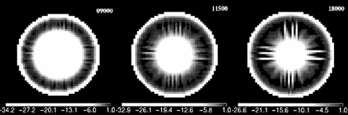
Fig. 5. Temperatures (°C) relative to the basal-melting point during growth sequence of the 228.15 K experiment using a rough bed. The introduction of the rough bed permits earlier separation of flow regimes and a more balanced piecewise instigation of the pattern.
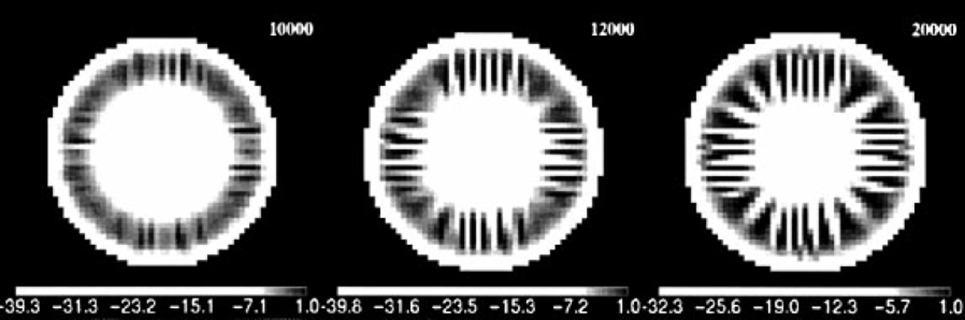
Fig. 6. Temperatures (°C) relative to the basal-melting point during growth sequence of the 223.15 K experiment using a rough bed. As in the warmer cash,flow separation can start earlier in preferred localities over the rough bed.
The natural width of streaming features
The initial runs presented have a grid resolution of 25 km. Here we examine the effect a finer model resolution. If the streaming areas are modelled at their "natural width" and spacing rather than at scales governed by the numerical scheme and grid resolution then the size and spacing of the features should be independent of the model resolution. Figures 7 and 8 show the same situation as the circular cooler case {ST = 223 K having beds with the same 10 m amplitude roughness as above, resolved at 12.5 km and 5 km horizontal grid spacing respectively.

Fig. 7. (a) Temperatures (°C) relative to the basal melting point for the 223.15 Kscenario, using a rough bed resolved at 12.5 km grid resolution, (b) Detail of flow vectors for the same case. The overall shape and scale of the ice sheet follows that of the 25 km resolution, but a further cold-based spoke is found in each quadrant.

Fig. 8. (a) Temperatures (°C) relative to the basal melting point for the 223.15 Kscenario, using a rough bed resolved at 5 km grid resolution, (b) Detail for the same case. Further additional spokes are found in comparison to the 12.5 km resolution model and now there is considerable variability in the exact size and shape of individual streams despite the overall consistency in the radial frequency of the pattern. Some evidence exists for further splitting of the flow regime lower down.
In the 12.5 km case a similar spoked pattern develops, but with about one more additional well-resolved spokes in each quadrant between the zones of more confused flow lying orthogonal to the grid. There is approximately the same proportion of colder to warmer area in the zone where the flow is most separated. Each shows a similar pattern with the colder spokes being relatively parallel-sided and the warmer, intervening areas, fanning out. This is a pattern one might expect with steeper gradients towards the margin; the total increase in ice flux is accommodated by increasing the area of faster flowing ice. This overall trend is further continued in the 5 km resolution of the model (Fig 8). At this resolution there are perhaps eight or nine well-resolved spokes in each quadrant. In this latter case, however, the situation becomes more complicated since there they vary more in size and there is an added tendency for additional bifurcation of individual spokes to occur. In the less-well resolved zones too, the separation of flow is more apparent in the upper part of the flowline, but has the tendency to break down towards the margin. Of further interest is that the frequency of cold/warm area spacing in the upper part of the separated flow zone is approximately mirrored lower down with additional separation of flow. As the overall radial flow diverges outwards, there seems to be a tendency to insert further streams at a similar frequency. In other words, streams seem to be inserted as a means of balancing flow over a given cross-sectional width. A slight suggestion of this also occurs in the 12.5 km resolution example.
Overall, an average "real" width of the colder, parallel spokes is roughly 100 km (4 gridpoints) in the 25 km resolution model, 70 km (6 gridpoints) in the 12.5 km model resolution and 60 km (12 gridpoints) in the 5 km resolution model. Although the scaling of the individually represented features changes it is clearly not some simple multiple of the grid spacing. The problem of poorly resolved flow in some zones in which flow is orthogonal to the grid
Response to Variations in Mass Balance
The idea that the density of the streaming pattern functions so as to regulate total ice flux is easily demonstrated by varying the mass-balance conditions used in the model. Keeping the same surface-temperature regime as before, and keeping the same gradient of mass balance, and zero mass-balance position, the maximum mass balance was restricted to 0.3 m a"1 and increased to 0.7 m a"1 for two additional experiments. In effect, this roughly equates to creating an ice sheet with a "dryer" and a "wetter" interior, but with a similar ablation zone. These experiments were resolved at 12.5 km resolution as above and are shown in Figure 9. Although these model ice sheets have the same surface-temperature regime, the model with the higher mass balance adjusts to the greater ice flux both by having a steeper profile overall and by increasing the area of flow reaching pressure-melting point. The reverse applies to the model with restricted mass balance. In this case, areas of faster flow only develop favourable positions orthogonal to the grid axes.

Fig. 9. Experiments with the same 223.15 K scenario resolved at 12.5 km resolution, but for maximum mass-balance constraints of 0.3 myr–1 (a) and 0.7 myr–1 ( b) The lowering and raising of the total mass throughput in each case is regulated by a corresponding decrease and increase in the total warm-based area.
Such behaviour is additionally shown in Figure 10. Here a parallel-sided equivalent to the radial model is developed for the colder surface-temperature parameterization, also with a rough bed but at 25 km resolution (Fig. 10a). In this case, because the mass-balance scheme determines that flow is directed principally along one model axis, parallel-sided warm and cold-based zones develop with an irregular spacing, but with an even frequency on average. Increasing (Fig. 10c) and reducing (Fig. 10d) the mass balance in the same manner as for the radial case above has a similar effect. Note too in these experiments that, although the flow is not divergent, as for the radial case, the streaming zones are marginally wider towards the zone of maximum ice flux and also tend to dissipate close to the margin. In each case, streams exist as features of varying resolution. Each also demonstrates more evidence of the flow variation being supported by an uneven surface profile than was the case for the radial model.

Fig. 10. Parallel-sided ice-sheet model experiments produced by operating the mass-balance variation in only one dimension. The central ridge logically connects to itself, (a) is equivalent to the radial 223.15 K scenario and (c) and (d) show corresponding increases and decreases in mass balance as in Figure 9a and b. Figure 10b is the identical situation to Figure 10a but with the introduction of sliding
Sliding Streams
The flow variation illustrated so far depends solely on enhanced deformation from thermal feedback. Sliding behaviour is introduced with a linear sliding law as in the EISMINT 2 cases. Basal sliding velocity, ui is given by
where α is ice density, g is gravity, H is ice thickness, h is bed elevation and i = x, y is horizontal distance. B is a parameter set arbitrarily here to 10−2, an order of magnitude higher than the EISMINT 2 scenarios and twice that used by Reference Payne and DongelmansPayne and Donglemans (1997). This produced quite strong sliding velocities 10 to 20 times higher than from deformation alone. An additional simplified constraint is that sliding only, but necessarily, begins when the basal ice reaches the pressure-melting point. This is recognized as being unrealistic in that it is firstly a gross simplification of the link between basal melting and sliding and secondly creates a potential sharp discontinuity in velocity between sliding and non-sliding areas. The emphasis here however is not to try and produce a truly realistic representation of the sliding process and sliding-non-sliding transition. It is instead to illustrate the effect of introducing a further efficiency in ice-mass evacuation on the temperature-flow feedback.
Figure 11 shows the onset of sliding streams during the model ice build-up using an identical rough-bedded radial model to those previously used (ST = 223 K), but with additional sliding. The ice builds in a similar way, but the moment the bed reaches pressure melting, the sliding-thermal feedback is sufficiently strong to establish narrow streaming features. Initially, the convergence of flow towards these lower-profiled streams is sufficient to prevent the appearance of other streams, but as the ice sheet builds further additional streams are introduced. These sliding streams also tend to become wider, accommodating greater flux toward the margin and they further bifurcate in some instances in their most distal reaches. With this strong sliding, the drawdown markedly affects the surface profile of the ice sheet. The more efficient ice evacuation means that fewer streaming areas are required to maintain total balance. Equally, these sliding streams require more ice to stay "switched-on".

Fig. 11. The introduction of sliding to the 223.15 K run over a rough bed resolved at 12.5 km. (a), (b) and (c) show the growth sequence before equilibrium is reached in (d). These sliding streams also show preferred orthogonal orientation and splitting in their lower parts, ( e) shows details of flow vectors which are an order of magnitude larger than those produced from the areas which do not slide. This results in the marked localized relative lowering of surface altitudes within the stream.
Just as with the deformation-only flow variations, the patterns produced are markedly aligned with the grid axes. These have a typical spacing, but are random depending on the exact location of the initial streams. This effect is best shown in Figure 12, which displays three identical models to the above (resolved at 25 km), but with different random bed roughness. Each model produces between six and eight streams, having a similar area occupied by streaming flow, although organized differently. The overall scaling is markedly similar to the finer resolution case.
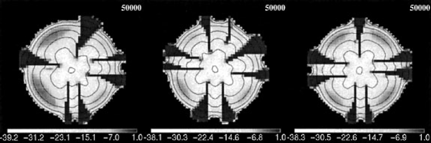
Fig. 12. Sliding resolved for three sliding cases using different rough beds at 25 m resolution. The precise patterning is different, but similarities in the overall scale and structure of the solutions are maintained.
Finally, the effect of introducing sliding can also be readily observed in a parallel-sided situation in Figure 10b, whose non-sliding equivalent is in Figure 10a. Again the streams are irregularly located but with a characteristic spacing overall. The more efficient sliding flow reduces these features to single cell-width entities in this case.
Discussion
We suggest that our results further demonstrate that the principal mechanism for establishing self-organized patterns of flow is the need for the ice-sheet system to produce a total-flow regime, impossible to maintain homogeneously in certain phases of thermomechanical flow. Colder (very cold) surface conditions will permit the ice flow in which steeper profiles maintain a cold bed without allowing creep feedback to start. In warmer regimes, ice profiles can be sustained in which basal pressure melting is met along all flowlines. In intermediate conditions, the only way for the ice mass as a whole to maintain balance is to support simultaneously areas in which both flow phases are found. The response of the ice mass to changes in surface temperature or mass balance in these circumstances is to change the total area drained by one flow system or the other.
The results (Figs 7 and 8) suggest that the scaling of the self-organized pattern is to some degree independent of the model resolution used. In the case of the experiments without sliding, the modelled stream features in the 25,12.5 and 5 km resolutions only vary in size by a factor of two at most. At the same time, these cases are resolved progressively by more gridcells. This concurrency points to some large-scale physics being a prime influence rather than the precise nature of the numerical implementation. This suggests that there is a tendency to produce streams of a given natural size and frequency, for a particular thermal and mass-balance condition. In addition, the introduction of the stochastically rough bed adequately demonstrates that minor variations in the precise scale of features can occur whilst a greater overall structure to the pattern exits. Despite the obvious simplifications of the sliding scheme used, it demonstrates that, if sliding also occurs, similar feature scaling is likely to take place.
In reality, local topographic variation and pre-existing forms are likely to have a strong influence on the precise nature of the pattern, fostering the formation of streams into suitable depressions (e.g. Reference Shabtaie and BentleyShabtaie and Bentley, 1987). But it is possible that not every depression can support persistent streaming flow and that the scaling of streaming patterns in response to larger-scale ice-sheet dynamics can exert an influence on the scales of glacially eroded landscapes. As suggested by Reference Payne and DongelmansPayne and Donglemans (1997), where flow becomes more confined such regulation is more likely to be facilitated by temporal oscillations in streaming.
A major problem remains with the numerical discretization of the thermodyamical equations presented here. The numerical method seems to fail when the flowlines run orthogonal to the grid axes. Gridpoint-by-gridpoint variability exists across the main flowlines, a problem which becomes more obvious at the higher resolutions. This suggests that artificial diffusion processes in the numerical scheme may be helping to smooth the flow in the streams which lie across the axes. On the one hand, we can observe that the structure of the streaming areas becomes more sharply resolved at finer grid resolutions. On the other hand, whilst there is no linear relation between the stream size and model resolution, the modelled stream sizes are clearly not independent of the chosen model resolution. There is a relatively sharp discontinuity between the warmer and colder areas and it may be the inability of the model to resolve the streaming/non-streaming boundary correctly that introduces the stream-size dependence on grid resolution. It is thus quite probable that the sizing of the modelled streams is strongly controlled by the numerical solution, but the precise mechanism for this is not understood at this point. The orthogonality of the solutions is not merely a relict of initial conditions since the minor irregularities or the roughened beds have a visible influence during ice growth. The initial influence of the irregularly roughened beds on the streaming is insufficient to overcome the tendency to structure the solution parallel to the grid axes. The problem increases in regions of greater ice flux. Whilst our approach has improved the resolution of the flow patterns better, these more sharply illustrate the deficiencies of the model. In particular they are highlighted by the idealized scenarios used. Further work is required to fully understand and overcome them.
Conclusions
Overall, we do not suggest that we are correctly representing real streaming processes, nor that our modelled streams are indicative of any precise natural scales for ice streams. Rather, we suggest that the results show the tendency of some ice-sheet systems to separate and self-organize into regions of colder/slower and warmer/faster flow as a way of regulating their global ice-flux requirements. This separation is intimately related to creep instability which potentially may be further enhanced by meltwater-sliding feedback. Whilst the models may not be capturing the scale and patterning of such streams correctly, because of difficulties in the numerical scheme, we suggest that they point to the existence of real analogues of the larger-scale dynamic. In the same way that we may pose the question as to why a certain density of stream network exists in a fluvial system, we may ask what processes cause a certain density of ice streams to occur within an ice sheet. In part this relates to the influence of the underlying local topography, but in part also it relates to the ability of the whole system to maintain particular flow regimes with the available mass.
Higher-resolution models, which employ a stochastic element, may improve the representation of ice-stream features in idealized conditions. The inclusion of a thermally dependent sliding mechanism tends to concentrate the number and size of flows for a given mass-balance regime, but consistency in number and patterning of the sliding zones also exists.
Acknowledgements
We gratefully acknowledge the support of NERC grant GS2/02/1463 in facilitating this research, particularly the development of high-performance computing techniques used to produce the higher-resolution solutions.


