


INTRODUCTION
Glaciers in mountainous regions and the associated meltwater runoff are particularly sensitive to climatic changes (e.g. Zhou and others, Reference Zhou, Kang, Gao and Zhang2010; Engelhardt and others, Reference Engelhardt, Schuler and Andreassen2015). Most glaciers around the globe have been shrinking since the end of the Little Ice Age with increasing ice loss rates since the early 1980s (Bolch and others, Reference Bolch2012; IPCC, Reference Stocker, Qin, Plattner, Tignor, Allen, Boschung, Nauels, Xia, Bex and Midgley2013). Despite different local conditions and response times, glaciers all over the world show to a large extent a uniform retreat (WGMS, Reference Zemp, Roer, Kb, Hoelzle, Paul and Haeberli2008, Reference Zemp, Nussbaumer, Naegeli, Gärtner-Roer, Paul, Hoelzle and Haeberli2013; Zemp and others, Reference Zemp2015).
Glaciers accumulate water as snow and ice during the cold or wet season, and release it as meltwater during the dry or warm season, when water demand is largest in the downstream areas (Casassa and others, Reference Casassa, López, Pouyaud and Escobar2009). In regions where meltwater during summer is an important source for irrigation systems, power production or even drinking water, changes in the regional water cycle may affect agricultural land and threaten the livelihood of populated areas downstream (Kaltenborn and others, Reference Kaltenborn, Nellemann and Vistnes2010; Kaser and others, Reference Kaser, Grohauser and Marzeion2010). Glacier retreat and changes in the associated streamflow are therefore expected to have great socioeconomic impact on regions that are dependent on meltwater from glacierized areas like in the Himalayan mountains (e.g. Sharma and others, Reference Sharma, Vorosmarty and Moore2000; Bolch and others, Reference Bolch2012; Immerzeel and others, Reference Immerzeel, Pellicciotti and Bierkens2013). In various mountain regions, extensive glacio-hydrological research has already been carried out, including the Alps (e.g. Oerlemans, Reference Oerlemans2000), Norway (e.g. Engelhardt and others, Reference Engelhardt, Schuler and Andreassen2014), the Andes (e.g. Favier and others, Reference Favier, Wagnon, Chazarin, Maisincho and Coudrain2004; Gurgiser and others, Reference Gurgiser, Marzeion, Nicholson, Ortner and Kaser2013; Nicholson and others, Reference Nicholson, Prinz, Mlg and Kaser2013), the Tibetan Plateau (e.g. Mölg and others, Reference Mölg, Maussion, Yang and Scherer2012) and the Nepalese Himalaya (e.g. Kayastha and others, Reference Kayastha, Ohata and Ageta1999). However, very few investigation have been carried out in the Indian part of the Himalaya so far (Koul and Ganjoo, Reference Koul and Ganjoo2010; Azam and others, Reference Azam2014a). Limited access to restricted areas and sparse observations are the reasons for the large uncertainties connected to recent glacier volume and mass changes in the Hindu Kush Himalayan (HKH) region (Hewitt, Reference Hewitt2005; Bolch and others, Reference Bolch2012; Kääb and others, Reference Kääb, Berthier, Nuth, Gardelle and Arnaud2012; Gardelle and others, Reference Gardelle, Berthier, Arnaud and Kb2013).
Snow- and glacial melt contribution can be quantified by calculating the residual of the water-balance equation (e.g. Kumar and others, Reference Kumar, Singh and Singh2007). However, in the HKH region runoff measurements are sparse and access to available observations is limited due to governmental policies. The identification of glacier responses to climatic changes and associated feedbacks over these large and remote areas is needed to quantify the glacier contribution to water resources (e.g. Immerzeel and others, Reference Immerzeel, Pellicciotti and Bierkens2013; Koldunov and others, Reference Koldunov2016). Glacier mass-balance and runoff models are therefore necessary for long-term glacier mass-balance simulations and estimation of the associated runoff at high altitudes, as well as to provide the past, present or future relation between glaciers and climate.
Runoff processes in the Himalaya are complex. The glacier meltwater contribution is important especially during warm and dry years (e.g. Naz and others, Reference Naz, Frans, Clarke, Burns and Lettenmaier2014). In addition, the response of glacier-fed streamflow to climatic changes is difficult to estimate due to the opposing trends of increasing glacial melt and decreasing glacier areas (e.g. Soncini and others, Reference Soncini2015). The impact of the ongoing climate change (Vaughan and others, Reference Vaughan, Stocker, Qin, Plattner, Tignor, Allen, Boschung, Nauels, Xia, Bex and Midgley2013) will initially increase melt and discharge. Eventually, the reducing glacier areas will limit the water supplies of downstream communities, resulting in more frequent water shortages during the dry season. Meltwater is extremely important for the Indus basin (Immerzeel and others, Reference Immerzeel, van Beck and Bierkens2010), and it is one of the river systems that will most likely experience substantially reduced water availability due to shrinking glaciers (Rees and Collins, Reference Rees and Collins2006). Such changes in runoff have already been observed, but there is still large uncertainty regarding when increased glacial melt will not compensate the reduced glacier areas (Xu and others, Reference Xu2009).
We present a modeling approach to calculate the mass balance of Chhota Shigri Glacier and meltwater runoff in the period 1951–2099. The glacier is located in the upper Indus river system, and represents the Western Himalayan region (Ramanathan, Reference Ramanathan2011). We build on a previous study (Engelhardt and others, Reference Engelhardt2017), yet focus on the future evolution of glacier mass-balance, runoff and glacial melt contribution to runoff. The simulations are forced by high-resolution meteorological variables for the period 2015–99, from two climate scenarios (representative concentration pathway (RCP) 4.5 and RCP 8.5), while the glacier area is annually updated from 1951 until the end of the 21st century.
METHODS
Study area
Chhota Shigri (32.28°N, 77.58°E) is a north-facing valley glacier, located on the Pir Panjal Mountain Range in the Indian state of Himachal Pradesh in western Himalaya (Fig. 1). With a glaciated area of ~16 km2 (in the year 2000) and a catchment area of ~35 km2 (Wagnon and others, Reference Wagnon2007; Ramanathan, Reference Ramanathan2011), almost 50% of the study area is covered by glaciers. The glacier length is ~9 km and covers an elevation range from 4050 to 5830 m a.s.l. The main flow and the glacier tongue of Chhota Shigri have a northerly orientation, but the tributaries in the accumulation area have various orientations. However, the glacier consists of two main flows, of which the larger one is coming from east. Debris covers 3.4% of the glacier surface area (Vincent and others, Reference Vincent2013), and is mainly situated in the lower ablation area (<4500 m a.s.l.). The debris cover consists of particles of various sizes, ranging from a few millimeters to several meters. The surface slopes range between 10° and 45° and the glacier tongue is situated in a narrow valley. Runoff from the catchment collects in a single proglacial stream contributing to Chandra River, which is one of the tributaries of Chenab River in the Indus river system.

Fig. 1. Left: Landsat-8 OLI image from 28 September 2014 showing the catchment of Chhota Shigri Glacier (red contour) based on Wagnon and others (Reference Wagnon2007) and the glacier area (green contour). The inset picture shows the location of the study area (red star) in the Chenab River basin in North India. Right: Elevation of Chhota Shigri Glacier in 500 m contours using SRTM data.
Chhota Shigri is situated in the monsoon-arid transition zone between two distinct precipitation regimes: the Mid-Latitude Westerlies (MLW) and the Indian Summer Monsoon (ISM) (Bookhagen and Burbank, Reference Bookhagen and Burbank2010; Azam and others, Reference Azam2014a). Most of the precipitation occurs during the accumulation season (October–May) due to the MLW; in the hydrological year 2012/13, the ISM contributed only ~12% to the annual precipitation, with the majority being supplied by the MLW, as revealed by a precipitation gauge (Geonor T-200B) at Chhota Shigri Base Camp (3880 m a.s.l., L-BC in Fig. 1). In the same period, at a meteorological station at Bhuntar airport (situated ~50 km south-west from Chhota Shigri, at 1092 m a.s.l.), the ISM contributed almost 50% of the annual precipitation (Azam and others, Reference Azam2014b). The more pronounced ISM signal in Bhuntar compared with the area of Chhota Shigri glacier illustrates the need of locally adjusted precipitation values.
At Chhota Shigri glacier, in-situ surface mass-balance measurements have been carried out annually since 2002 (Ramanathan, Reference Ramanathan2011), and are the longest series of continuous mass-balance observations available in the entire Himalayan region (Azam and others, Reference Azam2016). According to these observations, the average annual glacier-wide mass balance between 2003 and 2014 is –0.56 (±0.40) m w.e. a–1. In situ geodetic measurements by Vincent and others (Reference Vincent2013) between 1988 and 2010 revealed a moderate mass loss over that period of –3.8 (±2.0) m w.e., corresponding to –0.17 (±0.09) m w.e. a–1. Further, Azam and others (Reference Azam2014b) reconstructed the annual mass balances of Chhota Shigri glacier for the period 1969–2012, using the long-term meteorological measurements from Bhuntar airport, and obtained on average –0.30 (± 0.36) m w.e. a–1.
To represent the study area in a modelling approach, we used the glacier outlines from the Global Land Ice Measurements from Space (GLIMS) glacier database (Raup and others, Reference Raup2007). For the year 2000, the outline of Chhota Shigri glacier in the database is 14.7 km2. In this study, two adjacent glacierized areas of together 1.5 km2, which are contributing to the outflow of the main glacier, were considered part of Chhota Shigri glacier. For the runoff calculations, the modeled catchment area comprised both the glacierized and non-glacierized areas upstream from the discharge station. The catchment area of the study was 34.8 km2, which corresponds to a 46.5% glacierized area in the year 2000.
The elevation of the model area was taken from a DEM, which was derived from the Shuttle Radar Topography Mission (SRTM) data of the USGS (http://earthexplorer.usgs.gov). The DEM is available at a resolution of 1 arcsec (≈30 m).
Forcing data
Meteorological forcing for our study were daily 2 m air temperature and precipitation values from regional climate models (RCMs) that were driven by global weather reanalysis (ERA-Interim) or General Circulation Models (GCMs). In order to cover a very long study period, we used output of three different RCMs with increasing horizontal resolution to cover period 1951–2099 (Table 1).
Table 1. Overview of the available regional climate model time series
Both the Rossby Centre regional atmospheric climate model version 4 (RCA4) and the REgional atmosphere MOdel (REMO) time series are covering the Coordinated Regional Climate Downscaling Experiment (CORDEX, http://www.cordex.org) South Asia domain (see Kumar and others, Reference Kumar2015). The performance of REMO in this region has already been evaluated in several studies (e.g. Jacob and others, Reference Jacob2012; Saeed and others, Reference Saeed, Hagemann and Jacob2012; Kumar and others, Reference Kumar2015). The Weather Research and Forecasting (WRF) Model (version 3.7.1) calculations were performed over a domain centered on Chhota Shigri glacier. The RCA4 used GCM output as forcing (from MPI-M-MPI-ESM-LR historical scenarios), and REMO was forced by the ERA-Interim reanalysis time series (Dee and others, Reference Dee2011). WRF was run with a nested approach with 5 km grid spacing for the inner domain and 25 km grid spacing for the outer domain. The latter was also forced with the ERA-Interim reanalysis time series.
The horizontal interpolation of the RCM time series to each grid point of the mass-balance model was achieved by linear horizontal interpolation of the values from the four closest RCM grid points to each grid point of the mass-balance model. The vertical adjustment of the temperature and precipitation time series over the whole model domain was performed by using the monthly average temperature lapse rates and precipitation gradients of the respective RCM output.
To calibrate the obtained temperature and precipitation time series, we performed a bias correction. First, the horizontally interpolated and vertically adjusted WRF temperature and precipitation values were corrected with in-situ observations from the automatic weather station (AWS) and the precipitation gauge, respectively. For temperature, the correction uses the bias between the monthly average temperatures from the RCMs and the observed monthly average temperatures of the period of available temperature measurements (2010–13). For the the average annual air temperature the temperature bias between the WRF time series and the measurements (RCM minus observations) is − 2.6°C. After the calibration of the high resolution WRF time series, the homogenization of the other two RCM time series was carried out by a bias correction so that the monthly average temperatures within the overlapping periods (i.e. 2009–14 between REMO and WRF and 1989–2005 between RCA4 and REMO) are in agreement.
A similar approach was performed for precipitation based on its measured annual total in the hydrological year 2012/13, the only year of available precipitation observations. Since only 1 year of precipitation measurements was available for this study, this observed annual precipitation was used for calibration instead of monthly values. The precipitation bias between the WRF time series and the measurements was –0.191 m w.e. a–1 or –18% of the annual precipitation sum. However, the average WRF precipitation distribution throughout the year follows the precipitation pattern of a measurements in Kaza (Tawde and others, Reference Tawde, Kulkarni and Bala2016), located ≈50 km east of Chhota Shigri and in the same valley (Lahual Spiti valley), north of the orographic barrier, as the outflow of Chhota Shigri.
For the 2015–99 period, high resolution (5 km grid spacing) future climate scenario time series were generated by using the newly developed Intermediate Complexity Atmospheric Research (ICAR) Model (Gutmann and others, Reference Gutmann, Barstad, Clark, Arnold and Rasmussen2016). ICAR is a 3-D, quasi-dynamical, linear climate model. Essential input variables are 3-D outputs from RCMs or reanalysis as input. Required information is temperature, pressure, water vapor mass-mixing ratio and horizontal wind components. Optional variables include the hydrometeor fields, incoming short-wave and long-wave radiation and skin temperature of water bodies. The ICAR model uses wind fields from a linear, mountain-wave theory to calculate perturbations to the wind velocities. This wind field is used to advect heat and moisture instead of solving the Navier-Stokes equations of motion, as used in many other atmospheric models. By eliminating the Navier-Stokes calculations, the ICAR model can run several orders of magnitude faster than regular atmospheric models (Gutmann and others, Reference Gutmann, Barstad, Clark, Arnold and Rasmussen2016). The computational time can be further minimized by reducing the number of model layers.
The Thompson Microphysical Scheme (Thompson and others, Reference Thompson, Field, Rasmussen and Hall2008) was used to obtain realistic precipitation estimations and the Noah land surface model (Niu and others, Reference Niu2011; Yang and others, Reference Yang2011) is used to estimate temperature and humidity at the surface. Since ICAR is a quasi-dynamical, linear model and not a full atmospheric model, the typically biased, calculated precipitation needs some adjustment. We used the 2009–14 results from the high-resolution WRF time series (5 km grid spacing; forced by ERA-Interim) as reference to estimate the precipitation bias-correction fields in ICAR. These bias correction fields were applied on the time series of the future climate scenarios. The precipitation bias was estimated at 0.13 m w.e. a–1 (12%).
For the future climate scenarios, we used output from the Norwegian Earth System Model (NorESM) that is based on the Representative Concentration Pathways (RCP) 4.5 (the so-called climate stabilization scenario) and RCP 8.5 (Van Vuuren and others, Reference Van Vuuren2011). The variables were first dynamically downscaled to 25 km by using REMO and then further dynamically downscaled to 5 km by using ICAR.
The historical time series (1951–2014) consist of the downscaled output from the three described RCMs (Table 1), i.e. RCA4 from 1951 to 1988, REMO from 1989 to 2009, and WRF from 2009 to 2014. Combining the historical time series and the two future climate scenarios (2015–99) results in daily temperature and precipitation values for a 149-year long simulation period (1951–2099). The annual temperature of the historical RCM output within the domain of the mass-balance model ranges between –9.8 and − 5.5°C (Fig. 2a). Likewise, the annual precipitation rate ranges between 1.278 and 2.605 m w.e. a–1 (Fig. 2b). About 20–25% of the annual precipitation occurs between June and September, and can be attributed to the ISM. The remaining ~80% occurring between October and May can be attributed to MLW. The RCP 4.5 climate scenario does not predict a change in average precipitation over time. The RCP 8.5 climate scenario time series predict a slight decrease of annual precipitation by 5% compared with the historical values (1951–2014). Annual air temperature that already depicted a strong increase in the historical time series, keeps increasing in both climate scenarios (Fig. 2a). This temperature increase is similar for both climate scenarios until ~2050. After that, the RCP 8.5 climate scenario shows a continued temperature increase, whereas the temperature increase in the RCP 4.5 climate scenario slows down such that the temperature curve flattens out towards the end of the 21st century.
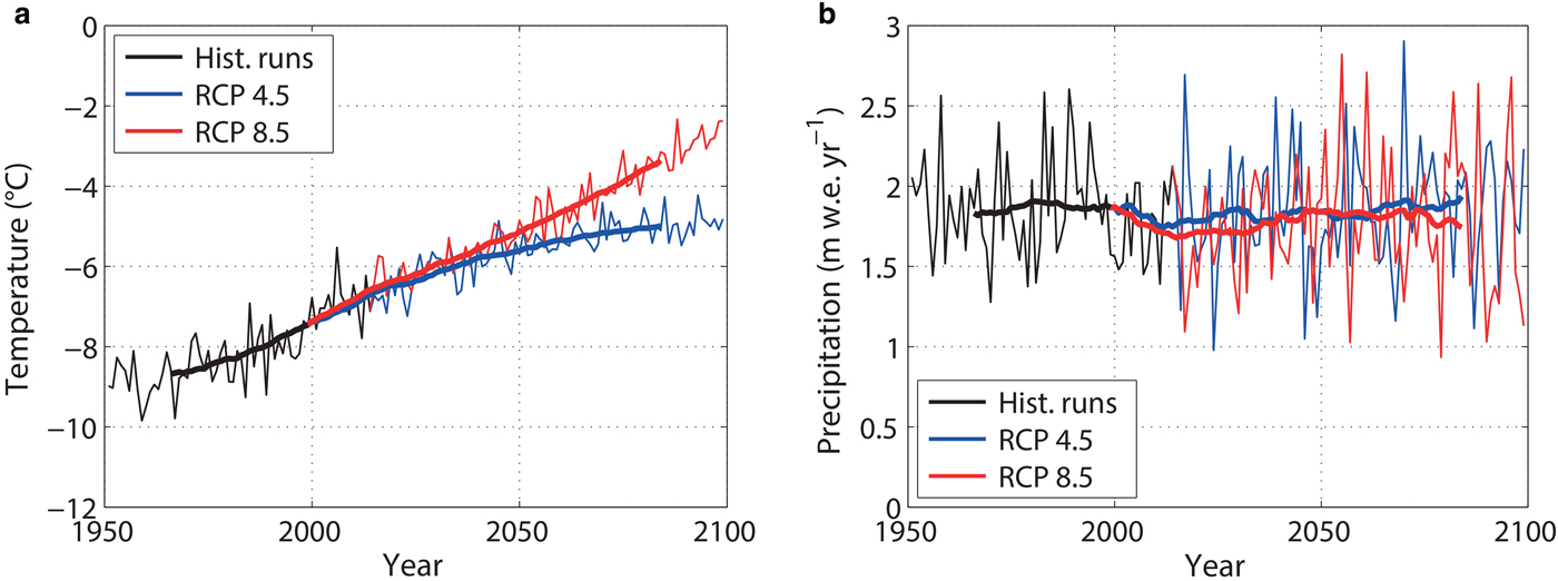
Fig. 2. Annual air temperature (a) and annual precipitation (b) from the model input, averaged over the model domain. The historical values (black) for 1951–2014 are followed by the 2015–99 future projection, based on RCP 4.5 scenario (blue) and RCP 8.5 scenario (red). Annual values are presented by thin lines, whereas the bold lines represent the 31-year moving average.
Mass-balance model
A mass-balance model, with a horizontal grid resolution of 10 arcsec (≈300 m), was used to calculate the surface mass balance in the catchment of Chhota Shigri glacier (34.8 km2). The model uses as input daily temperature and precipitation values at each model grid point. The simulations were performed for the period of available meteorological input (1951–2099), individually for all grid points representing an area that is at least partly inside the model domain. The glacier area during the model period was updated annually using an ice dynamics model (described in the section ‘Ice dynamics model’). Precipitation was accumulated as snow when the air temperature was lower than the threshold temperature for snowfall (T s), which was set to 1.3 ( ± 0.5)°C. Following Kienzle (Reference Kienzle2008), we applied a linear transition interval of 2°C where the precipitation gradually shifts from snow to rain. Daily melt of snow or ice M snow/ice was calculated when the air temperature was above the threshold temperature for melt (T m), which was set to − 1.9( ± 0.6)°C, using a distributed temperature-index approach including incoming short-wave radiation (see Pellicciotti and others, Reference Pellicciotti2005):
 $$M_{{\rm snow}/{\rm ice}} = \max [C \cdot (T - T_{\rm m}) + R_{{\rm snow}/{\rm ice}} \cdot I,0],$$
with the melt factor C, the air temperature input T, the radiation coefficients R for snow and ice and the potential direct solar radiation I. Following Hock (Reference Hock1999), potential solar radiation was calculated at each grid point within the model domain. The calculation of I accounted for slope, aspect as well as shading effects from the surrounding topography inside and outside the model domain, and was computed on each day of the year. The use of potential solar radiation allows to account for melt events due to high solar radiation intensity at temperatures close to the freezing point. In order to retrieve the seasonal mass balances from the daily mass-balance series, we defined the beginning and end of each season respectively as the day when the glacier-wide mass balance was at its annual maximum (end of the winter season) and at its minimum (end of the summer season). The calibration of the model is based on the available annual mass-balance measurements (2003–14), and was validated with geodetic measurements and other model approaches from various time periods, as described in Engelhardt and others (Reference Engelhardt2017). The five model parameters (Table 2) were optimized to achieve best the agreement between simulated and observed annual mass balances. A Monte-Carlo simulation with 10 000 independent runs allowed the model parameters to vary within a plausible range. We assumed as uncertainty of each model parameter their value range determined by the best 100 simulations.
Table 2. Average and uncertainty of the five model parameters
Runoff model
Runoff was calculated as the sum of glacial melt (ice melt and firn melt), snowmelt (both inside and outside the glacier area) and liquid precipitation (rain) for the whole catchment (Eqn (1)). Each runoff component as well as the combined runoff were calculated on a daily time step individually for each grid point of the model domain. The daily simulated discharge integrated over the whole model domain (R) was calculated as the sum from all grid points.
 $$\eqalign{R = & \underbrace{{M_{{\rm ice}} + M_{{\rm firn}}}}_{{{\rm glacial \;melt}}} + \underbrace{{M_{{\rm snow\; on\; glacier\; area}} + M_{{\rm snow\; outside\; glacier\; area}}}}_{{{\rm snow\; melt}}} \cr & + M_{{\rm rain}}},$$
The model does not include a water retention factor (which delays the onset of runoff) or storage constants for snow, firn or ice (which smoothes runoff over some days) as in Engelhardt and others (Reference Engelhardt, Schuler and Andreassen2014), since runoff and the runoff components were evaluated monthly or annually. Annual runoff was calculated for calendar years in order to capture the runoff of the whole ablation season.
Ice-dynamics model
The ice dynamics were simulated with a 1-D ice flow model that has been used in several studies (e.g. Oerlemans, Reference Oerlemans1986; Stroeven and others, Reference Stroeven, van de Wal, Oerlemans and Oerlemans1989; Greuell, Reference Greuell1992). Since Chhota Shigri glacier has a complex geometry with several tributary glaciers, we divided the glacier into six basins. The ice flow was calculated along each of the six central flowlines of the glacier basins. One flowline is located on the ice body that flows down the main glacier valley. The other five flowlines were defined on the tributaries to the main flow.
The model resolution on each flowline is 50 m. At every grid point, the ice flow through a vertical cross section S was calculated based on the conservation of mass:
 $$\displaystyle{{\partial S} \over {\partial t}} = \displaystyle{{\partial (US)} \over {\partial x}} + w_{\rm s}b,$$
where U is the vertically averaged ice velocity of a cross section, w s is the width at the glacier surface, and b is the specific mass balance. The cross sections were parameterized with a trapezoid defined by a constant effective slope of the valley walls λ and a valley width w 0, such that the area of the cross section S is given by:
 $$S = H\left( {w_0 + \displaystyle{1 \over 2}\lambda H} \right).$$
By combining Eqns (3 and 4), we obtained the ice dynamics in terms of the time evolution of the glacier ice thickness (H) along the 1-D glacier flowline:
 $$\displaystyle{{\partial H} \over {\partial t}} = \displaystyle{{ - 1} \over {w_0 + \lambda H}}\displaystyle{\partial \over {\partial x}}\left\{ {HU\left( {w_0 + \displaystyle{1 \over 2}\lambda H} \right)} \right\} + (w_0 + \lambda H)b.$$
The ice velocity U is the sum of the deformation velocity U d and the sliding velocity U s. We used the shallow ice approximation (SIA) such that the ice velocity was determined by the local driving stress and we assumed that the ice is at the pressure melting point, as melt may occur over the whole glacier. Then the vertical averaged ice velocity is given by
 $$\eqalign{U & = U_{\rm d} + U_{\rm s} \cr & = f_{\rm d}H\left( {\rho _{{\rm ice}}gH\displaystyle{{\partial h} \over {\partial x}}} \right)^3 +\; f_{\rm s}\displaystyle{{{\left( {\rho _{{\rm ice}}gH(\partial h/\partial x)} \right)}^3} \over H},}$$
with ice density ρ
ice, gravitational constant g and ∂h/∂x for the glacier surface slope. The values for parameters of deformation f
d = 1.9 × 10⁻²⁴ Pa−3s−1 and sliding $f_{\rm s} = 5.7 \times 10^{ - 20}\,{\rm P}{\rm a}^{ - 3}{\kern 1pt} {\rm m}^{ - 2}{\kern 1pt} {\rm s}^{ - 1}$
were taken from Budd and others (Reference Budd, Keage and Blundy1979). The sliding parameter f
s includes the bulk effect of the water pressure on glacier sliding and the model did not include seasonal variation in velocity. Combining Eqns (5 and 6) gave an expression for the evolution of the ice thickness that was solved with a forward explicit scheme on a staggered grid, in times steps of 5 h.
$f_{\rm s} = 5.7 \times 10^{ - 20}\,{\rm P}{\rm a}^{ - 3}{\kern 1pt} {\rm m}^{ - 2}{\kern 1pt} {\rm s}^{ - 1}$
were taken from Budd and others (Reference Budd, Keage and Blundy1979). The sliding parameter f
s includes the bulk effect of the water pressure on glacier sliding and the model did not include seasonal variation in velocity. Combining Eqns (5 and 6) gave an expression for the evolution of the ice thickness that was solved with a forward explicit scheme on a staggered grid, in times steps of 5 h.
Following Zuo and Oerlemans (Reference Zuo and Oerlemans1997), the contribution of the tributaries to the main flowline was calculated by converting the ice flux from the tributary into an elevation change of the main flowline. The ice flux of the tributary was calculated at the last tributary gridpoint that has a higher surface elevation than the main flowline at the point where the two meet.
The 1-D model was forced by annual surface mass balances. We derived a linear mass-balance gradient β and a time-dependent equilibrium line altitude (ELA) for each of the glacier basins from the 2-D mass-balance model results for the reference surface. To account for the elevation-mass balance feedback, the specific mass balance b at a gridpoint with surface elevation h was then given by
 $$b = \beta (h - {\rm ELA}).$$
The mass-balance model provided the ELA for the period 1952–2099. As model spin-up, the forcing until 1951 was chosen such that the simulated glacier extent in 2000 matched the observed glacier outline in that year.
As the glacier bed topography is unknown, we reconstructed the glacier bed from the mismatch between observed and modelled surface topography in an iterative procedure (Leclercq and others, Reference Leclercq, Pitte, Giesen, Masiokas and Oerlemans2012; van Pelt and others, Reference van Pelt2013). The simulation is a transient run until 2000, and then the bed was adjusted by half the difference between modelled and observed surface elevation. The first iteration started in 1800 with zero ice thickness, subsequent iterations started in 1900. In the period 1952–2014 the mass balances were calculated from the annual ELA. Before 1951, the model was forced with an ELA history that makes the simulated glacier area agree with the observed glacier area in year 2000. The iterative procedure was performed until further bed elevation updates did not improve the simulated surface elevation.
The future glacier evolution was calculated by forcing the ice-dynamics model with the ELA derived from the surface mass-balance model, which was forced with the RCP 4.5 and RCP 8.5 scenarios for the period 2015–99. The spin-up of the model was initiated in 1702. Thereafter the model was run with the modelled ELA from 1952 to 2099.
To validate the obtained glacier areas, we manually derived the outlines of the glacier extents from a Landsat image (from August 1977) and a from a Sentinel image (from October 2016). Both images were downloaded from the USGS Glovis (https://glovis.usgs.gov).
RESULTS
Glacier area and volume
The simulated glacier geometry and surface velocity agree well with the observations by Azam and others (Reference Azam2012), who measured ice thickness and surface velocity at four cross sections on the main flowline. Our modelled maximum ice thickness does not fit very well to the observations at every cross section (Fig. 3), which can be ascribed to the parametrization of the bed geometry with a trapezoid. The agreement between observed and modelled cross-sectional area is good, and the modelled value is within the measurement uncertainty on three of the four cross sections. Also, the modelled surface velocity is close to the observed surface velocity. As the modelled cross-section area and the velocity are close to the observations, the modelled ice flux seems to correspond well with the real ice flux. The results revealed only small area changes for Chhota Shigri glacier in the period 1951–2014, which corresponds with observed area change for the period 1977–2016 (Fig. 4a).

Fig. 3. Simulated maximum ice thickness, glacier cross sections and surface velocity along the main flowline, compared with results by Azam and others (Reference Azam2012).

Fig. 4. Simulated glacier area (a) and glacier volume (b) using input from historical time series for 1951–2014 (black) and input from RCP 4.5 (blue) and RCP 8.5 (red) scenarios for 2015–99.
The uncertainty of the validation data is approximately in the same range as the area mismatch. The uncertainty in the Landsat images from 1977 is larger than the uncertainty of the Sentinel image from 2016, due to much lower resolution in the Landsat images. Forced by the climate scenarios RCP 4.5 and RCP 8.5, the model predicted a decrease of the glacier area in the period 2015–50 of ~1 km2 for the RCP 4.5 scenario, and ~2 km2 for the RCP 8.5 scenario. A strong decrease of glacier area was predicted in the period 2050–99, however with large differences between the two used climate scenarios: a decrease of 35% to ~10 km2 for the RCP 4.5 scenario and a decrease of 70% to <5 km2 for the RCP 8.5 scenario.
The reduction of the glacier area is a consequence of the simulated decrease in glacier volume (Fig. 4b). The modeled reduction in glacier volume was even stronger than for the glacier area, with a glacier wastage of ~70% (RCP 4.5) to 90% (RCP 8.5) by the end of the 21st century relative to the year 1950.
Glacier mass balance
The simulated mass balances for Chhota Shigri glacier in 1951–2014 are similar to the results of Engelhardt and others (Reference Engelhardt2017), where the same data input was used but who applied a constant glacier surface (reference surface) for the entire period. In the period 2015–99, the simulated mass balances show little differences between the two climate scenarios (Fig. 5). However, with a negative annual mass balance average of –0.4 (±0.3) m w.e. a–1, the glacier area continues to shrink until the end of the model period.

Fig. 5. Simulated seasonal and annual glacier mass balances of Chhota Shigri using input from historical time series for 1951–2014 (black) and input from RCP 4.5 (blue) and RCP 8.5 (red) scenarios for 2015–99, based on annually updated glacier areas. Annual values are presented by thin lines, whereas the bold lines represent the 31-year moving average.
Negative mass balance and the shrinking glacier area were due to an increasing average ELA during the simulation period (Table 3). In the last three decades, the ELA has already increased from 5011 m a.s.l. (1951–80) to 5054 m a.s.l. (1981–2010). However, the further increase of the ELA is dependent on the climate scenario. The RCP 4.5 scenario suggests a moderate increase of the ELA to about 5100 m a.s.l. (2011–40) and 5200 m a.s.l. (2070–99). The RCP 8.5 scenario suggests higher ELA by 50 m in 2011–40 and a further increase by 250 m in 2070–99, resulting in ELA as high as 5400 m a.s.l.
Table 3. 30-year averages, averaged over the whole catchment area of Chhota Shigri glacier, of glacier area and its relative extend in the catchment, average equilibrium line altitude (ELA), simulated annual mass balances (B a), annual temperature (T a), annual precipitation (P a), summer (June–September) precipitation (P s) and its contribution to annual precipitation)
Runoff
The average annual runoff show a large interannual variability with values between +1.3 and +2.6 m w.e. a–1 (Fig. 6a). Average runoff in the historical simulation increased from the period 1951–80 to 1981–2010 from 1.86 (±0.2) to 2.05 ±0.2) m w.e. a–1. Thereafter, and until the end of the future projection, annual runoff remained rather constant at ~2.0 (±0.2) m w.e. a–1, independent of the climate scenario (Table 4). In both climate scenarios, the average contribution of snowmelt to annual runoff increases from 50 in the historical simulation to more than 60% for 2011–99 (Table 4), but shows more interannual variability, especially in the RCP 8.5 scenario (Fig. 6a).

Fig. 6. (a) Annual runoff, snowmelt (middle curve), and glacier melt (lower curve), and (b) August runoff, and glacier melt in 1951–2099. The simulations are based on input from historical time series (black curves) and from climate scenarios RCP 4.5 (blue curves) and RCP 8.5 (red curves) for 2015–99. Annual values are presented by thin lines, whereas the bold lines represent the 31-year moving average.
Table 4. 30-year averages of simulated annual runoff, annual runoff sources, August runoff and August glacial melt for the catchment of Chhota Shigri glacier
After an initial increase, the glacial melt contribution reaches a peak in the period 1981–2040 (Fig. 6). Then it decreases from ~30 to 20% by the end of the simulation period. However, this decrease is simulated to occur earlier for the RCP 8.5 scenario where the decrease is already evident during the period 2041–70 (Table 4). For the RCP 4.5 scenario, the decrease in glacial melt contribution is not visible before the 2070–99 period.
August runoff increased by 0.5 m w.e. a–1 until ~2030 (Fig. 6b). Thereafter, August runoff was simulated to decline. This decline is more pronounced in the RCP 8.5 scenario. The glacier contribution to runoff in August is ~50% (Table 4), but shows a high interannual variability.
Annual runoff remains rather constant during the simulation period. However, there is a visible shift of runoff towards earlier in the year (Fig. 7). July runoff peaks at ~6–7.5 m w.e. a–1 in all periods and both climate scenarios. The largest percental changes however are evident in May. In this month, the RCP 4.5 scenario suggests a doubling of the monthly runoff from ~1 to 2 m w.e. a–1, and results with the RCP 8.5 scenario shows even a tripling with more than 3 m w.e. a–1 in the period 2070–99. A similar runoff increase was simulated for June. In the historical simulation, runoff was ~3 m w.e. a–1. In both climate scenarios, runoff was simulated to increase to ~5 m w.e. a–1. In July, the RCP 4.5 scenario suggests an almost constant runoff of ~7 m w.e. a–1. Using RCP 8.5 scenario, a slight increase in the period 2011–40 is followed by a decrease until the end of the simulation period. After 2070, runoff is modeled to a level below current values. For August and September, a decrease in monthly runoff was modeled in both climate scenarios. The decrease is most prominent in August when the RCP 8.5 scenario suggests a decrease from 6.6 (2011–40) to 4.7 m w.e. a–1 by the end of the simulation period (Fig. 7b).

Fig. 7. Monthly runoff (solid lines) and from glacial melt (dashed lines) in (a) the RCP 4.5 scenario, and (b) the RCP 8.5 scenario, averaged over five 30-year periods between 1951 and 2099.
DISCUSSION
The parameter of this study were taken from Engelhardt and others (Reference Engelhardt2017), where they were calibrated by the available glacier mass-balance measurements (2003–14) and validated both by geodetic measurements for different time periods, and by runoff measurements (2010–13). The uncertainty to the regional climate model input was also evaluated in the study Engelhardt and others (Reference Engelhardt2017) by modeling mass balance and runoff for the periods where there is overlapping meteorological input available. The uncertainty of the glacier mass balances due to differences among the RCM time series was calculated to 0.32 m w.e. a–1 between the RCA4 and REMO time series, and 0.11 m w.e. a–1 between the REMO and WRF time series. The uncertainty to the model parameter was calculated to 0.08 m w.e. a–1. The runoff uncertainties due to differences among the RCM time series were calculated to ±0.1 m w.e. a–1 and $ \pm 5\% $
for the contributing sources. Additional uncertainties due to the model parameters are ~±0.1 m w.e. a–1 for each of the average annual runoff values and ~
$ \pm 5\% $
for the contributing sources. Additional uncertainties due to the model parameters are ~±0.1 m w.e. a–1 for each of the average annual runoff values and ~ $ \pm 3\% $
for the contributing sources.
$ \pm 3\% $
for the contributing sources.
Further uncertainty is related to long simulation and the importance of local effects on temperature lapse rate or precipitation gradients (Mandal A, Ramanathan A, Engelhardt M and Nesje A, unpublished) that might not be represented sufficiently in the RCM output. The temperature and precipitation gradients were directly retrieved from the RCM output, which could have led to inaccuracies of local mass-balance gradients.
The low melt threshold factor (T m in Eqn (1)) of − 1.9 (± 0.6)°C reflects the typical situation of many areas in the Himalayan mountains where melt occurs on days with positive temperatures during daytime, while daily average temperatures are yet below freezing point. The need for a lower melt threshold temperature in these situations was also discussed by van den Broeke and others (Reference van den Broeke, Bus, Ettema and Smeets2010) conducted for western Greenland, where it was suggested to use threshold temperatures down to −5°C.
Uncertainty is also related to the temperature and precipitation input in the years 1951–88, which only were available at 50 km horizontal resolution that is too coarse for brief precipitation events to be resolved adequately. These time series are based on a global climate model and not on ERA-Interim reanalysis time series. Due to the large overlapping period of 17 years (1989–2005) with the REMO data that are based on ERA-Interim, we achieved a suitable bias correction of these input time series. The small change in annual precipitation over the simulation period is in line with other studies for the Western Himalayan region (e.g. Dimri and Dash, Reference Dimri and Dash2012). However, Immerzeel and others (Reference Immerzeel, Pellicciotti and Bierkens2013) concluded that the largest future runoff uncertainty is due to uncertainties in projected precipitation. The stochastic nature of the meteorological variables is a larger source of uncertainty for average runoff than the uncertainty of the RCM output in the future (Ragettli and others, Reference Ragettli, Pellicciotti, Bordoy and Immerzeel2013).
A rising ELA implies that more of the winter accumulation is melting during summer, leaving less snow behind that can form firn and new glacier ice that eventually flows down to the ablation area. The large increase in the ELA in this study is in line with the results of Soncini and others (Reference Soncini2015) in the Karakoram area. Changes in glacier mass balance by this study are related to changes in temperatures, which are expected to increase by 2.6°C (RCP 4.5) or 4.3°C (RCP 8.5), whereas annual precipitation remains almost unchanged (Table 3).
The negative annual glacier mass balance in the period 1951–2015 indicates that the glacier is already not in equilibrium with current climate conditions. Even with a smaller area loss of 35% using the RCP 4.5 scenario (the so-called climate stabilization scenario), the glacier ice volume will greatly decrease by 80% until the end of the century. The effect of debris cover on glacier area changes is not considered. However, Chhota Shigri is a clean glacier compared with other glaciers in the Himalayan mountains (Ramanathan, Reference Ramanathan2011), with only the lower parts of the glacier tongue (≈3% of the glacier area) covered by debris. Since thin debris cover enhances, while thicker debris cover prevents melt (Scherler and others, Reference Scherler, Bookhagen and Strecker2011), the long-term evolution of glacial melt and corresponding glacier area changes might diverge from the model results.
Immerzeel and others (Reference Immerzeel, Pellicciotti and Bierkens2013) calculated an increase in meltwater runoff for two watersheds in the Western and Eastern Himalaya at least until 2050. Our results do not show such an increase for the annual runoff sums during the 21st century (Fig. 6a). August runoff peaks already in the period 2011–40 with both a slightly higher peak and a stronger decline after 2040 for the RCP 8.5 scenario (Fig. 6b). This change in runoff contribution is due to a shift of meltwater production towards less glacial melt and increased snow melt. With increased air temperatures in all months, the onset of snow melt occurs earlier in the season. Decreased glacier area provides less glacial melt in late summer when less snow is available for melt.
The high interannual variability of glacial melt in August illustrates the balancing effect of a glacier within a catchment. Annual total runoff shows much lower variability (Fig. 6b) since glacial melt is higher in warm and dry summers, and lower in cool and wet summers. A further decrease in glacier area however will eventually result in more variable annual runoff, and especially more variable late summer runoff.
CONCLUSION
The mass balance of Chhota Shigri glacier and runoff in its catchment area were simulated in the period 1952–2099. The average annual mass balances of Chhota Shigri were calculated to on average negative (–0.4 ± 0.3 m w.e. a–1) for the whole model period. Annual runoff was calculated to on average ~2.0 (±0.2) m w.e. a–1.
Average annual precipitation did not change much during the simulation period, but average annual air temperature increased by ~3.7°C (RCP 4.5) or 5.4°C (RCP 8.5). This led to a decrease in glacier area and to an increase in runoff in early summer, and a decrease in runoff later in the year as less glacial melt occurs. According to these results, especially in late summer runoff becomes more vulnerable to variations in summer temperatures and summer snowfalls, which alter the contribution of glacial melt to runoff.
The retreating glacier will show a major change in seasonal meltwater runoff. A continuation of the surface mass-balance measurements is therefore essential, since longer time series of uninterrupted measurements will improve model calibration. There is also a necessity to extend the model approach to other glaciers in the region since the simulation of glacier mass balance and runoff for larger regions is essential to estimate future evolution of the runoff regime further downstream close to settlements and agricultural areas in the coming decades.
CONTRIBUTION STATEMENT
Markus Engelhardt designed the study, performed the mass-balance and runoff calculations, and wrote the paper. Paul Leclercq performed the glacier response calculations contributed to writing the paper. Trude Eidhammer and Roy Rasmussen provided the WRF time series, Pankaj Kumar provided the REMO time series and Oskar Landgren provided the RCA4 time series.
ACKNOWLEDGEMENTS
We thank Scientific Editor Carleen Tijm-Reijmer and three anonymous reviewers who have significantly improved this paper. The study was part of the GLACINDIA project, funded by the Norwegian Research Council. This study was partially supported by the funding from the Federal Ministry of Education and Research, Germany, for the GLACINDIA project (contract 033L164) and REMO simulations were performed at the Climate Computing Center Germany (DKRZ). We thank Nikolay Koldunov from the Climate Service Center Germany for valuable input. We acknowledge the World Climate Research Programme's Working Group on Regional Climate, and the Working Group on Coupled Modeling, former coordinating body of CORDEX and responsible panel for CMIP5. We also thank the climate modelling groups (listed in the Methods) for producing and making available their model output. High performance computing support for the WRF simulations was provided by NCAR's Computational and Information Systems Laboratory, sponsored by the US National Science Foundation (NSF). Paul Leclercq was funded by the European Research Council under the European Union's Seventh Framework Programme (FP/2007–2013)/ERC Grant Agreement No. 320816. We also acknowledge the Earth System Grid Federation infrastructure an international effort led by the US Department of Energy's Program for Climate Model Diagnosis and Intercomparison, the European Network for Earth System Modelling and other partners in the Global Organisation for Earth System Science Portals (GO-ESSP). The Landsat-8 OLI data, courtesy of the US Geological Survey, was downloaded from EarthExplorer.


 Open access