


1. Introduction
In this paper we describe results of the compilation of data on Antarctic ice-sheet surface morphology, bedrock configuration, and ice thickness, based on data obtained primarily from airborne RES although other sources are used where appropriate. Knowledge of these three parameters has increased measurably since the last symposium on Antarctic glaciology In 1968. Whereas oversnow traverses conducting barometric altimetry and seismic shooting were typical of the 1950s and 1960s, airborne RES and satellite systems are currently employed.
Maps depicting ice-sheet morphology, bedrock configuration, and ice thickness are to be printed in colour and published as part of an Antarctic glaciological and geophysical folio by the Scott Polar Research Institute (SPRI) In 1982 (Reference Drewry and JordanDrewry and Jordan 1980, Drewry in press).
2. Radio echo-sounding (RES)
50% of the Antarctic ice sheet (6.8 × 10⁶ km2) has been surveyed during the last decade on a 50 to 100 km square grid using airborne RES techniques in a SPRI-US National Science Foundation (NSF)-Technical University of Denmark (TUD) programme. Descriptions of the technique and systems have been given elsewhere (Reference Evans and SmithEvans and Smith 1969, Reference RobinRobin 1975, Reference Skou and SØndergaardSkou and Sondergaard 1976, Reference ChriStensenChristensen 1970, Reference Drewry and MeldrumDrewry and Meldrum 1978, Reference Drewry and CracknellDrewry 1981). Pertinent to this study are the methods of reduction of data to achieve accurate surface and subgladal elevations. A flow chart outlining the reduction process is shown In Figure 1.

Fig.1. Flow chart for reduction of RES data. Crosswind and temperature corrections were applied to 1974–75 data only.
2.1. Navigation
All flights in this study were conducted using one or two inertial navigation systems (INS) of Litton LTN-51 type. Output from the INS (latitude, longitude, drift angle, heading, track angle, ground speed) were recorded either on punched paper tape (1971–72, 1974–75 seasons) or on magnetic tape (1977–78, 1978–79 seasons) at a sampling interval (bearing in mind a typical ground speed of 100 m s−1) of one data frame every 20 s (1971–72), 15 s (1974–75), 0.125 s (1977–78), and 0.25 s (1978–79). A data-logging system developed by the US Naval Weapons Center and made available by NSF was used during the latter two seasons.
Flight tracks derived from INS records have been adjusted to close all available fixes (e.g. terminal fixes, overflown bases and camps, mountains etc., of known position). Although errors between fixed and unfixed track positions are distributed linearly, such a simple treatment is not ideal due to the complex nature of INS (Reference Kayton, Kayton and FriedKayton 1969) but the small number of fixes on any one flight prevents a more sophisticated distribution of errors. Errors may arise from linear components, oscillating Schuler frequency elements with perturbations introduced by various aircraft manoeuvres. Rose (unpublished) gives a resume of these factors. The small number of fixes on any one flight prevents a more sophisticated distribution of errors.
It is possible to use ice thickness data at the intersection of two different flight lines to deduce the shift necessary for thicknesses to correlate (see Rose unpublished):
where hn(p) is the ice thickness of flight n at position p, Pn is the position at crossing point on flight n, and pn is the error in crossing point position on flight n.
In general there will be very many possible solutions to Equation (1). Rose found that for West Antarctica a mean shift of flight lines by 2.5 km would remove errors at 40% of crossing points, and this distance represents a lower bound for such navigation errors. The maximum difference on all Antarctic RES tracks was typically of the order of 8 km with RMS deviation over a whole flight of 4 to 5 km. In general, therefore, the error in navigation should be <<5 km anywhere, corresponding to less than 1 mm at a mapped scale of 1:5 000 000
2.2. Ice thickness
Aircraft terrain clearance and ice thickness are determined from RES records of echo delays. Received signals on Z-scope traces are usually enhanced by differentiation of signal strength with respect to time. Weak bottom echoes are also enhanced by the integrating effect of slowly moving film and a high pulse repetition frequency (PRF) typically in the order of 15 to 25 kHz. Digitization of records gives rise to certain random errors (from equipment and operator inaccuracies). Repeat measurements of a given distance displacement reveal an RMS deviation equivalent to 0.17 µs (25.5 m in air and 14.3 m in ice) (Steed unpublished). Oscillograms produced by a Honeywell 1856A Visicorder during the 1977–78 and 1978–79 seasons allowed improved digitization with RMS deviation of 0.12 µs (18 m in air and 10.1 m in ice).
Propagation velocity of radio waves in air is 300 m µs−1. Velocity in ice is related to relative permittivity ε'. Early estimates from laboratory studies suggested ε' = 3.17±0.07 within the frequency range 10 to 105 MHz (Reference Robin, Evans and BaileyRobin and others 1969). This value of ε' gives a velocity v = 169±2 m µs−1. More recent laboratory work, specifically at 60 MHz, shows a slight decrease in ε' with temperature but no detectable change with uniaxial compressive stress and resulting plastic flow (Reference Johari and CharetteJohari and Charette 1975). A value of 168 m µs−1, accurate to about 1%, is suggested by all these results. An interferometric log of a bore hole on Devon Island, NWT, Canada, by Reference RobinRobin (1975) gave a velocity of 167.7±0.3 m µs−1 at 440 MHz. Reference Shabtaie, Bentley, Blankenship, Lovell and GassettShabtaie and others (1980) have used a value of 173 m µs−1 for conversion of travel times at Dome C in East Antarctica
Higher velocities occur as the radio wave passes through low density snow and firn (Reference Shabtaie and BentleyShabtaie and Bentley (1982). Reference Robin, Evans and BaileyRobin and others (1969) derived a general solution to correct for this layer by inspection of several depth-density curves which resulted in the addition of an extra delay equivalent to a column of ice of thickness 10 m. This is estimated to be accurate to within 5 m for all types of firn.
All ice thicknesses reported here have been derived using v = 168 m µs−1 + 10 m (firn correction factor).
2.3. Altimetry
Altitudes of the ice-sheet surface and subglacial bedrock are determined relative to aircraft height by static pressure measurements using a pressure transducer (Garrett) with a maximum instrumental error of 22 Pa and an RMS error of 16 Pa (equivalent to 2.5 m). The major sources of error in determining aircraft barometric elevation arise from spatial and temporal changes in constant pressure surfaces associated with with weather systems: variations of up to 150 m over distances of a few hundreds of kilometres can occur (Steed unpublished). A “crosswind” correction (Rose unpublished) has been applied to some data since the geometrical height of a constant pressure surface will vary (assuming that winds are purely geostrophic). The correction also depends on aircraft latitude, velocity, and drift angle, and accumulates with time during the flight. For 1974–75 data the mean maximum crosswind correction was 83±3 m. On flights where transducer output was calibrated against aircraft pressure altimeters, corrections are necessary for the departure of the Antarctic atmosphere from the International Standard Atmosphere (ISA). ISA temperature at sea-level is 15°C, much warmer and less dense than in the Antarctic. Corrections were made based upon the ratio of mean temperature of the actual and ISA air columns, and typically in the range –50 to –150±15 m (Rose unpublished).
Even after application of these corrections icesurface elevations will differ at the intersection of two independent flights. Reference Jankowski and DrewryJankowski and Drewry (1981), for instance, found a mean error at crossover points of 47±44 m RMS. In order to minimize and redistribute these errors at nodes of the flight line grid and take account of alimited number of control elevations (e.g. geoceiver stations, sea-level, etc.) in producing new surface altitudes a random walk procedure has been employed. The mean elevation value at any one node will, after many thousands of visits during walks which begin and end at control points, converge on a stable solution as errors are redistributed over the whole grid. The results of this procedure were confirmed by a least-squares technique on the same data-set performed by the UK Directorate of Overseas Surveys.
Large-scale systematic errors of the RES survey altimetry after corrections and minimization are estimated for areas well away from control points to be significantly less than 50 m.
3. Antarctic coastline
There have been considerable improvements in the mapping of coastal areas of Antarctica in the last decade resulting especially from the use of satellite imagery (Reference SwithinbankSwithinbank 1974, Reference MacDonald, Williams and CarterMacDonald 1976, Reference Swithinbank, Doake, Wager and CrabtreeSwithinbank and others 1976). During the compilation of base-map data for the Antarctic glaciological and geophysical folio it was found necessary to produce an up-to-date coastline. The most recent and reliable charts of coastal areas were digitized to produce a coastal outline data base consisting of some 225k points. In some areas the coast was completely remapped using Landsat images fixed to geodetic ground control. This was undertaken between 120°E and 157°E, along the front of the Ross Ice Shelf and Filchner-Ronne ice shelves. While improvements will continue to be made in the coastal outline of the continent the present map is a reasonably accurate and up-to-date representation.
Table 1. COMPARISON OF LENGTHS AND FREQUENCY OF COASTAL TYPES AROUND ANTARCTICA
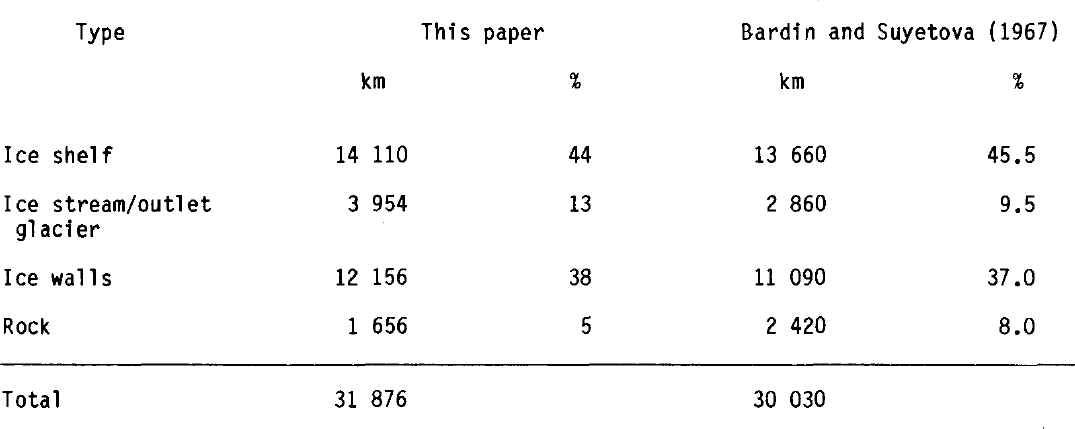
Using this new coastline data base it has been possible to recalculate the lengths of coastline occupied by ice shelves, outlet glaciers/ice streams, ice walls, and rock outcrops to provide comparison with the pioneering study by Reference Bardin and SuyetovaBardin and Suyetova (1967). Our results are given in Table I.
4. Ice-sheet surface
Ice-sheet surface elevations have been contoured at 100 m intervals from 101 000 SPRI RES determinations. TWERLE balloon altimetry (made available by courtesy of Dr Nadav Levanon (Reference Levanon, Julian and SuomiLevanon and others 1977, Reference Levanon and BentleyLevanon and Bentley 1979, Reference LevanonLevanon 1982), numbering some 5 000 points was also added to the data set as were geodetic satellite measurements and selected barometric altimetry from some oversnow traverses. All data were plotted at a compilation scale of 1:3 000 000. RES data were colour-coded and parameter-annotated along flight lines (see Reference DrewryDrewry 1975[a]). All other elevation values were plotted to three significant figures. Contouring was then undertaken, independently and by hand, by three persons, results compared, and a final version produced. In mountainous terrain (Transantarctic Mountains, Dronning Maud Land, Prince Charles Mountains, parts of Byrd Land) contours at 500 m were taken from the Soviet 1:3 000 000 map of Antarctica (Ministerstvo Morskogo Flota SSSR 1975). For contours in the Antarctic Peninsula the latest British Antarctic Survey (BAS) maps were used (British Antarctic Survey 1979, Directorate of Overseas Surveys 1981). The resulting ice-sheet surface map will be printed in colour at a scale of 1:6 000 000 in the forthcoming Antarctic glaciological and geophysical folio. Figure 2 presents a small-scale surface map using an interpolation procedure based on a 50 km sided matrix. Figure 3 is an isometric view of the ice-sheet surface. Between June and October 1978 a 13.5 GHz radar altimeter was flown aboard the satellite Seasat at a mean altitude of 800 km. The inclination of the satellite orbit of 108° resulted in coverage of coastal areas of Antarctica (to latitude 72°S). The altimeter had a precision of ~100 mm but due to the footprint size (12 km) over rough, sloping ice terrain and problems with interpretation of returned radar waveforms this was degraded to between 1 and 5 m. Analysis of derived surface altitudes by Reference Zwally, Bindschadler, Thomas and MartinZwally and others (1982) reveals a pattern for coastal East Antarctica which substantiially confirms the contours in Figure 2.

Fig.2. Contour map of the surface of the Antarctic ice sheet based upon RES, TWERLE, and some traverse data using a simple cubic interpolation and a matrix of size 50 km. Note that the lowest contour Is 200 m and the coastline (except edge of major ice shelves) is not shown. The detailed contour map will be published at a scale of 1:6 000 000 (Drewry 1n press).

Fig.3. Isometric view of the surface of the Antarctic ice sheet, based upon 50 km square matrix. Mountainous areas have been omitted. Note the steepness of coastal areas of the ice sheet, the effects of some of the large drainage basins (e.g. Lambert Glacier) and subtle surface relief.
5. Ice-sheet thickness and ice volume
All RES ice thickness data (SPRI and selected other sources) have been combined with existing depth determinations from seismic shooting to produce a contour map for the whole continent. As a result it has been possible to derive estimates for the volume of ice in Antarctica. Volume is given by:
where h is the ice thickness and a is the area.
The problem is to find a satisfactory method of estimating Equation (2). Several techniques are available. A contour map of ice thickness enables the area occupied by each ice-thickness band to be specified and used in construction of a hypsometric curve which may then be integrated to give ice volume. An alter7 native method, which has been adopted in this study, is to use equally spaced ice-thickness data points, averaged within each cell of a matrix of arbitrary size superimposed over Antarctica and taking account of ice in ice-shelf and grounded-ice areas. Where no measured values are available an estimated value based on adjacent or regional values has been specified. Total volume is then the sum of all the cell volumes:

where Δi is mean ice volume in cell of unit area.
A further method assumes that since the RES grid covers a very large proportion of the area of West Antarctica and over a third of East Antarctica the values taken by the means of all RES determinations within these areas will be representative of the larger region. The product of regional areas and average ice thickness yields the volume. Corrections can be made for areas of outcrop, and any bias in RES depths towards shallower thicknesses (i.e. thickest ice may not be recorded). Continental volume is then:

where Ag is area of grounded ice including ice rises, Ai is area of ice shelf, Am is area occupied by rock outcrop, hg is mean thickness of grounded ice, hi is mean thickness of ice shelf, and Q is correction factor for shallow ice bias in measurement. This has been derived using the ratio of RES flight track where bed echoes were not recorded due to system performance limitations to track with detectable bed returns. Major subscripts refer to East Antarctica: e, West Antarctica: w, Ross Ice Shelf: r, Filchner-Ronne ice shelves: f, Antarctic Peninsula: p, and mountain or rock outcrop: m.
Space does not permit the detailed tabulation and comparison of the results of these two methods (Equation (3) and Equation (4)) but a difference of less than 2° was found. We have listed some of the results calculated using Equation (4) which provides a natural breakdown for the principal regions of Antarctica (Table II). The total volume of ice is found to be just over 30×106 km3.
Table II. Area, ice thickness, and ice volume for antarctic ice sheet (Equation (4))

5.1. Estimation of errors
The error associated with this calculation of total ice volume is estimated as ±2.5 × 10⁶ km3, made up of contributions from uncertainty in area and ice thickness measurements.
The area of Antarctica was determined using the coastline compilation discussed in section 3 projected on a Lambert azimuthal equal-area net at a scale of 1:6 000 000. A magneto-strictive digitizing system was employed which gave an accuracy better than 1% on repeated measurements of the same test areas. This figure of <1% embodies both machine and operator random errors. In view of the fact that mapping of the Antarctic coastline is of variable quality and many of the boundaries are highly mobile (i.e. the fronts of ice shelves and outlet glaciers) alikely error in measured sector areas is <3%. This would give rise to an uncertainty in calculation of total Antarctic ice volume of 1.0 × 10⁶ km3.
The ice thicknesses given in Table I I were derived from several sources (see notes for Table III) but primarily from RES measurements. Of critical importance in calculation of volume is the accurate assessment of the mean value for the larger areas such as East and West Antarctica. Just over one-third of East Antarctica is covered by RES grid. Some 28 500 equally-spaced ice-thickness determinations in this area were used to derive a mean value which was considered representative and applied to the whole region. Data from the limited number of oversnow traverses in that part of Antarctica not covered by dense RES grids show that the variations in ice thickness are similar to those observed from areas of RES coverage.
Since the ice sheet mantles a wide variety of subglacial topography the RMS deviation of thickness is high. The standard error of the mean (SEM) at the 99% level for the calculated thickness values is in the order of ±50 m. In West Antarctica where the RES grid gives very good coverage of the whole area the SEM is also ±50m.
An uncertainty of ±50 m in calculated mean thickness values for East and West Antarctica gives a combined uncertainty in ice volume of ±0.52 × 10⁶ km3. Taking into account extrapolation of the sample mean into areas of less or no measured data and Inspection of ice-th1ckness variations on available oversnow traverses suggest that ± 1 × 1 106 km3 might be a realistic error In estimates of the 1ce volume deriving from thickness uncertainty.
Table III Comparison of morphometric data for antarctic ice sheet

For the major ice shelves (Ross and Fllchner- Ronne) there 1s very good RES coverage and due to their relatively uniform characteristics the Icethickness means may be considered representative. SEM for the Ross Ice Shelf 1s, for example ±20 m. For the smaller ice shelves in East Antarctica, West Antarctica, and the Antarctic Peninsula thicknesses have been derived from a limited number of RES and seismic soundings and application of the relationship, determined by Reference Crary, Robinson, Bennett and BoydCrary and others (1962: fig.l4) from the Ross Ice Shelf, between observed surface elevations S and ice thickness h:
In general all ice-shelf thicknesses for these smaller shelves will lie between 100 and 500 m. Given a total area for them of 0.543 106 km2 the deviation in ice volume from that calculated using a mean based upon Equation (5) is not likely to be more than 0.2 × 10⁶ km3. In the Antarctic Peninsula a high proportion of terrain is ice-free (~20%) and elsewhere subglacial topography is extremely rugged. Although considerable RES has been conducted 1n the peninsula area there are only a few published sources of ice-thickness data (see Reference SwithinbankSwithinbank 1968, Reference SmithSmith 1972, Reference SwithinbankSwithinbank 1977, Reference CrabtreeCrabtree 1981). Nevertheless these have proved adequate for basic estimation of ice volumes within the gladerlzed (grounded ice) area (0.300 × 10⁶ km2). Uncertainty in average ice thickness as high as ±500 m would only change the continental ice volume by ±0.15 × 10⁶ km3. The total error in ice volume is thus the sum of these smaller contributions: ±(1.0 + 1.0 + 0.2 + 0.15), say ± 2.5 × 10⁶ km3.
5.2. Discussion of areas and ice volumes
Table III compares the data calculated in this paper with other recent compilations. In many cases it has proved impossible to compare results for subcontinental areas due to the lack of accurate definition of the regions used in published accounts.
The estimate of area of the conterminous Antarctic (I.e. including offshore islands joined by ice shelves) has not changed substantially 1n recent years. There is less than 0.5% difference between the Soviet figure accepted by Reference Aver'yanovAveryanov (1980) and that calculated here. As our errors in deriving areas are of the order of 1% the two figures may be taken as identical. Similar comments are applicable to the areas of grounded ice sheet and ice shelf. We believe, however, that the area of rock outcrop given by Reference KorotkevichKorotkevlch (1968), 0.03 to 0.04 106 km2, is too low and suggest a value an order of magnitude larger.
The considerably higher ice volumes (Table III) are due to greater values for ice thickness. All the previous estimates were based upon a total data set numbering some 1 500 unevenly scattered seismic reflection determinations and approximately 9 000 less reliable gravity observations. Continuous RES over half of the continent has now provided 77 000 digitized values from the SPRI programme alone. They indicate that average ice-thickness values are considerably in excess of previous estimates. It should also be borne in mind that comparison of RES with seismic-gravity ice-thickness measurements has revealed substantial underestimation of ice depths on several major oversnow traverses in East Antarctica (Reference DrewryDrewry 1975[b]).
It is interesting to note results for the two major ice shelves. Traditionally the Ross Ice Shelf has always been considered the larger. In terms of floating ice extent this is still true (compare 0.526 × 10⁶ km2 for the Ross Ice Shelf with 0.473 × 10⁶ km2 for the Ronne-Filchner ice shelves). The total area of the two ice shelves including all ice rises is now almost identical. This change comes as a result of refinement of the grounding line of the Ronne-Filchner ice shelves from satellite mapping and RES (Reference Swithinbank, Doake, Wager and CrabtreeSwithinbank and others 1976, Reference Drewry, Meldrum and JankowskiDrewry and others 1980). The Ronne-Filchner ice shelves possess considerably thicker ice than found in the Ross Ice Shelf, due principally to the flow constraint imposed by large ice rises distributed across the ice shelf: they inhibit large-scale creep-thinning and thicken ice up-stream. The thicker ice results in a total ice volume for the Ronne-Filchner ice shelves considerably in excess of the Ross Ice Shelf.
6. Subglacial bedrock characteristics
RES and all other available data on subglacial topography have been combined and contoured. In areas of high data coverage (i.e. parts of East and West Antarctica within the RES grid) the contour interval is 250 m. Elsewhere the contour interval is 500 m. Maps of selected regions have already been published (Reference Jankowski and DrewryJankowski and Drewry 1981, Steed and Drewry in press). The continental map depicting subglacial configuration will be published in the Antarctic folio at a scale of 1:6 000 000. In this paper we briefly discuss some of the broad characteristics of the data.
Figure 4 depicts histograms for RES-derived bedrock elevations in East, West, and for all Antarctica covered by RES grid (~50%). Gaussian functions (taking the same area and with sample RMS deviation) have been fitted to the frequency distributions. It can be seen that East Antarctic data conform closely to a normal distribution (a x2 test indicates that the observed and normal distributions are similar at the 99% level). The data for combined East and West Antarctica show similar statistical features. The West Antarctic histogram is more positively skewed and less “normal”. This is probably accounted for by failure of the RES system to detect deep bedrock in the vicinity of the Bentley Trough and parts of the Byrd subglacial basin. Ice thicknesses here are in excess of 4 km and two-way dielectric absorption high (up to 110 dB) as a result of warmer ice temperatures (mean annual surface temperature >–30°C). Nevertheless a x2 test indicates similarity with normal frequency curve at 95% level.

Fig.4. Histograms of the frequency distribution of bedrock elevations in (a) West and (b) East Antarctica (and (c) combined data). The curve for the normal frequency 1s given by:

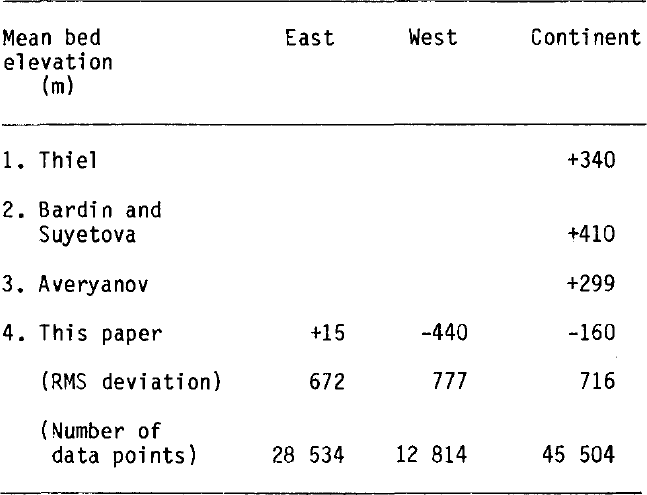
The Gaussian characteristics of the bedrock elevations enable several other studies to be undertaken which rely on this statistical assumption, such as the adjustment of elevations for the isostatic effects of superimposed ice load (Jankowski unpublished, Steed unpublished). Table IV summarizes the principal elements of the bedrock surface in Antarctica from SPRI RES data.
Table IV. Subglacial bedrock characteristics
Acknowledgements
The SPRI RES project was funded under UK Natural Environment Research Council (NERC) grant GR3/2291. Antarctic airborne field work was conducted under a collaborative programme with the US National Science Foundation and, since 1974–75, with the Technical University of Denmark. The generous logistics support by NSF and US Navy Task Force 199 and Antarctic Development Squadron (VXE-6) is gratefully acknowledged. Preparation of data for the Antarctic glaciological and geophysical folio is funded by NERC, British Petroleum, and Phillips Petroleum. We wish to thank Dr N Levanon who kindly made available TWERLE data. A P R Cooper assisted with computer processing of data and D Dickens and G Howard with aspects of data reduction.


