


1. Introduction
Heinrich events are sequences in the sedimentary record of the North Atlantic which indicate periods when large amounts of ice-rafted debris were scoured from Hudson Bay and Hudson Strait and transported out to the ocean on icebergs (Heinrich, 1988; Bond and others, 1992; Grousset and others, 1993). The simplest interpretation of these sequences (and others described by Bond and Lotti (1995)) is that they occur via repealed, quasi-periodic surges of the Laurentide ice sheet (Andrews and Tedesco, 1992; Clark, 1994), and specifically of the Hudson Bay ice dome draining through Hudson Strait. MacAyeal (1993) has suggested a simple mechanism whereby this could occur, and Fowler and Johnson (1995) have shown that this concept is compatible with theoretical descriptions of ice flow over wet, deformable sediment.
The concept of ice-sheet surges is highlighted by the existence of ice streams, for example in Antarctica, which are relatively fast outlet flows. Their notable feature, particularly on the Siple Coast, is their lateral variability. That is to say, the ice streams which drain into the Ross Ice Shelf divide the drainage basin into regions of fast and slow flow. This is suggestive of a lateral instability, as is also the fact that drainage of ice sheets generally seems to occur through localized ice streams. Again, a principal feature of the Siple Coast ice streams is that they may be underlain by a layer of wet, deformable sediment (Alley and others, 1987).
In this paper, we extend Fowler and Johnson’s (1995) crude model in two ways. First, we allow for spatial variation in the variables, thus deriving a non-linear diffusion-type equation, whose surging solutions we describe. Secondly, in laterally extensive flows (such as on the Siple Coast, for example), we allow for lateral spatial dependence of the variables and we show how the resulting model may result in the spontaneous generation of ice streams. Payne (1995) has also found oscillations in an ice-sheet model with thermally activated flow and sliding, although the mechanism is different from that proposed here. In other work, he also found that laterally extensive flows are subject to streaming instability (personal communication from A. J. Payne).
2. Ice-Sheet Model
We follow the development of Fowler and Johnson (1995), who described an approximate model of ice-sheet dynamics, based on the (asymptotic) limits of strong temperature-dependent variation of viscosity and small thermal diffusivity. We consider a two-dimensional ice sheet of thickness h(x, t) (x is flowline distance, t is time) undergoing plug flow: the horizontal velocity is u(x, t.), where u is just the sliding velocity, shearing is negligible and we are assuming that the bed is at the melting point, mainly for convenience.
Mass conservation implies
where a is the accumulation rate and subscripts x and t denote partial derivatives. The sliding velocity u is determined by a sliding law of the form prescribed by Fowler and Johnson (1995). If the basal shear stress is τ and the heat flux up into the ice (the basal cooling) is q, then the heat delivered to the interface is G + τu − q, where G is the geothermal heat flux. We assume if is constant, having a value G =0.05 W m−2. If the resulting water supply is distributed across a channelized system with inter-branch spacing w d , then the water flux per channel increases in the direction ni ice flow according to

where ρ w is water density and L is the latent heat.
Walder and Fowler (1994) developed a theory which implied that, for ice sheets moving over wet sediment, the effective pressure N (overburden ice pressure minus water pressure) would be related to Q by
where c* was given by
c′ ≈ 1.1 × 10⁴ bar

where values 0 < r, s < 1 are probably appropriate. The coefficient c is a constant which measures how “sticky” the bed is. High values of c mean that the bed has high friction. The shear stress is
and the cooling rate may be determined by a thermal boundary-layer analysis.
Specifically, the temperature T satisfies
where the base is taken as z = 0, κ is the thermal diffusivity and the vertical velocity is w = −zu′ = − z∂u/∂x by continuity (since u = u(x, t)). If uh 2 /κl ≫ 1, where l is the horizontal length scale, then it is appropriate to solve Equation (7) with
where T A is the prescribed surface temperature, which we lake to be constant. A similarity solution is appropriate and we find that the basal cooling is given by (Fowler and Johnson, 1995)

where ΔT = T M − T A , ρ is ice density, c p is the specific heat, k is the thermal conductivity and
The second term is added to represent conductive cooling when u → 0.
The seven Equations (1), (2), (3), (5), (6), (9) and (10) determine the variables h, u, Q, τ, g, N and ξ. We non-dimensionalize the variables by choosing scales [h], [u], etc., where we define

Here, we cheat a bit, because the values of c*, c and particularly w d are very uncertain, even if appropriate. Therefore, we argue as follows. A value of c can be inferred from present conditions on Ice Stream B, Antarctica, where τ = 0.15 bar, u = 500 m year−1, N = 0.4 bar (Bentley, 1987), thus

The value of c* is taken from Equation (4), choosing |h x | ~ 10−3, D s = 10−4 m. Thus,
We have no estimate of w d , so we use [N] = 0.4 bar n determine w d.We then find from Equation (11) that

where M = [a]l. We choose ![]() , rather arbitrarily, and for values
, rather arbitrarily, and for values

and c given by Equation (12), we find M = 4 × 10⁵ m2 year−1 and
We then have, with ρ w = 103 kg m−3, L=335 kJ kg−1, c p = 2 kJ kg−1 ‘Κ−1, ΔΤ = 50 Κ, k =1 W m−1 K−1, G = 0.05 W m−2,
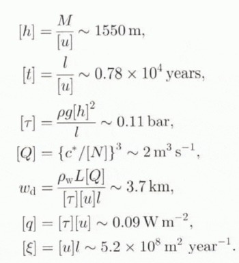
When the equations are non-dimensionalized with these scales, we obtain

where the parameters are defined by

The eq uations can be written in the form

where

It should be emphasized that the values of the parameters are not set in stone and we illustrate our thesis with differing values below.
3. Analysis
Fowler and Johnson (1995) analysed a parameterized version of Equation (20) by replacing derivatives by a heuristic integration. In effect, the second two equations and elimination of Q indicated that u(h) could be multi-valued. When Equation (20) 1 is solved with such a flux law, periodic surges result (on the convective time-scale, here ~8000 years). In this section, we explore how these results extend to spatially dependent versions of this model.

Fig. 1. Multi-valued velocity vs stress at values λ = 0, γ = 1.8, β = 3.7. This choice of parameters is distinguished from the estimates in Equation (19) by historical accident. In fact, by reseating u and τ in Equation (3.4), it is easy to show that the shape of the curve depends only on β/γυ, υ = (R + 2 − S)/2(R + 1) = 11/18 here. For Equation (19), β/γυ ≈ 1.7, while for the present values, β/γυ ≈ 6. Examination of other values suggests that F(τ) IS multi-valued approximately for β/γυ
![]()
were replaced by

First, we extend the model in Equation (20) to apply to an entire ice sheet with a single divide at x = 0. Evidently, we have

However, the model is most easily discussed for x > 0. We denote Equation (20) 2 as u = f(τ, Q), so that

where f τ = ∂f/∂τ, f Q = ∂f/∂Q. Since ξ and Q are essentially quadratures, this has the apparent character of a degenerate non-linear diffusion equation, since ∂f/∂τ > 0. The degeneracy refers to the vanishing diffusion coefficient when h = 0.
We discuss the full x-dependent model further in section 4; here, let us take a parameterized version of Equation (20), where we replace Q
x
by Q and ξ by u in Equation (20)
3. Then (with λ = 0) whence we have u = F(τ). It is easy to see by graphical considerations that F(τ) will typically be multi-valued since Q = τ
−R/S
u
![]() = τ
−s/3 (u
1/2)6r/s
, (Fig. 1). This is analogous to but more realistic than the parameterized model of Fowler and Johnson (1995) (who also took τ = h
2). The multi-valuedness arises through the conflicting roles of u in water production. A slow mode is possible where Q is small, because low Q means low u and also low u means cooling is effective at preventing much water production. However, at the same parameter values, it is possible to have high Q and high u. The large u is maintained by the high Q which is produced by frictional heating, cooling being less relatively effective at high u.
= τ
−s/3 (u
1/2)6r/s
, (Fig. 1). This is analogous to but more realistic than the parameterized model of Fowler and Johnson (1995) (who also took τ = h
2). The multi-valuedness arises through the conflicting roles of u in water production. A slow mode is possible where Q is small, because low Q means low u and also low u means cooling is effective at preventing much water production. However, at the same parameter values, it is possible to have high Q and high u. The large u is maintained by the high Q which is produced by frictional heating, cooling being less relatively effective at high u.


Fig 2. Schematic sequence of an ice-sheet surge following the semi-parameterized model (Equation (3.5)). In the quiescent phase, the ice sheet thickens (AB → A′B′) on the lower branch of the u vs τ curve. At B′, u jumps to the top branch and this region of fast flow propagates rapidly backwards to G, so that the activated region GH slumps forward. The resulting slump at G causes increased stress there and the surge region is likely to propagate backwards to F. Following the surge, the quiescent phase resumes.
What is the effect of this partial parameterization? From Equation (3.2), we have

whence

which is a non-linear convective–diffusion equation, with the distinguishing feature that dF/dτ = F′ < 0 on the middle branch of Figure 1: negative diffusion!
If the ice balance b(x) = ![]() a(x)dx is an increasing function, then (with h decreasing) b/h is also, and the steady-state solution of Equation (3.5), with hh
x
= −f
−1
(b/h), will have (moving outwards from the divide) three regions of slow flow (lower branch of Figure 1), transition (middle branch) and fast flow (top branch). Because of the negative diffusion, the transition region is violently unstable and the ice sheet must oscillate.
a(x)dx is an increasing function, then (with h decreasing) b/h is also, and the steady-state solution of Equation (3.5), with hh
x
= −f
−1
(b/h), will have (moving outwards from the divide) three regions of slow flow (lower branch of Figure 1), transition (middle branch) and fast flow (top branch). Because of the negative diffusion, the transition region is violently unstable and the ice sheet must oscillate.
For a marine ice sheet with b ≠ 0 at the margin, the shear stress is (formally) infinite (this is also true for a land-based ice sheet with b = 0 at the margin) and it is questionable whether the time-dependent problem is well posed. However, for the situation where the ice drains into an ice shelf, we will have b and h non-zero at the ice-sheet/ice-shelf transition and thus τ is finite there. We conjecture that the way in which the ice sheet oscillates is as follows. Let the values of τ at the lefthand and righthand noses of Figure 1 be τ − and τ + (τ − < τ +). If the ice sheet is shallow, we suppose τ < τ + everywhere. As the ice sheet thickens, τ increases until τ = τ + at the front. Then u jumps to the top branch by a rapid transient in the drainage system and we surmise that an “activation wave” passes upstream (Fowler, 1987), shifting the region with τ − < τ < τ + to the fast branch. The resulting activated ice now surges forward, lowering the ice thickness until the stress is lower than τ − everywhere. A repetition of the build-up can then occur. The sequence of events is portrayed in Figure We imagine that the advancing marginal ice pushes the ice shelf forward through compressive stresses, while the draw-down of the inland ice will cause migration backward of the activated region to the divide (or extensional failure and ice-cliff formation and collapse).
4. Ice Streams
We now return to the full one-dimensional model (Equation (20)). It is easy to compute the steady state and an example is shown in Figure 3. It should be noted

Fig. 3. Steady-state ice sheet from the full one-dimensional model (Equation (20)). The accumulation function a is taken as zero. Initial values are h = 2, ξ =0.1, Q = 0.1, u = 0.5 and parameter values are γ = 0.2, λ = 0.36. Note that h → 0 (so u, → ∞) in a finite distance.

then we see that the positive feed-back term τu, which produces the term −uh 2 f Q h x , may cause the advection velocity to be negative. It is plausible that this may lead to instability in the same sort of way as before. In this section, we propose a model to examine the effect of the possible instability in a laterally extensive flow.
In order to do this, we write the approximate drainage flux Q = (c*/N)3 in a suitable vector form. In the derivation of this relation (Walder and Fowler, 1994), one has that Q is proportional to the square of the hydraulic head gradient (which is roughly ρg sin α), where α is the ice-surface slope. However, a more accurate expression is ρg sin α + ∂N/∂x, so that the drainage law is more accurately

where ψ = 1/ρg sin α. An appropriate vector form of this is

where ![]() is a unit vector downslope. Since |ψ ∇N| ≪ 1, we approximate the downslope and cross-stream water fluxes as
is a unit vector downslope. Since |ψ ∇N| ≪ 1, we approximate the downslope and cross-stream water fluxes as

where y is the lateral space variable, Conservation of water flux now takes the form (in steady flow)

and, if we non-dimensionalize as before, but choosing Q ⊥ ~ ψ[N][Q]/d, and choosing a lateral space scale
then Equation (4.5) becomes

with

Equation (4.7) thus takes the diffusive form (Q ║ = Q)

with l = 400 km (appropriate to the Siple Coast area), [N] = 0.4 bar, ρ = 917 kg m−3, sin α = 10−3, then ψ ~ 0.11 Pa−1 m and thus d ~ 42 km, comparable to the width of ice streams.
The variation of Q with y suggests that we should also allow for lateral variation of h. Indeed, one can posit a model similar to Equation (4.9) for h based on an almost parallel flow but one then finds that the lateral diffusion coefficient for h is large, whence we can deduce (just us for a valley glacier) that h ≈ h(x, t) and thus mass conservation leads to the (dimensionless) relation
where L is the (sealed) width of the flow area and M* is the sealed mass flux. We are assuming a prescribed value of M* at x = 0 with no accumulation, so that the mass flux M* is constant in x. As before,

Insofar as parameterized versions of this model show some signatures of run-away associated with multiple steady states, we might expect an initially laterally inhomogeneous flow to develop “hot spots” as x increases, corresponding to ice streams.

Fig. 4. Formation of ice streams from a laterally non-uniform initial condition. The parameter value are γ = 0.2, β = 1, λ = 0.36 (which are more appropriate values for the Siple Coast ice streams) and the model is integrated forward with initial thickness of 1500 m and velocity 1 m year −1 . The initial condition for Q is critical and is taken (dimensionlessly) as Q = 0.05 with five perturbations superimposed. The precise location and number of the ice streams generated depends sensitively on the initial prescription of Q chosen but the streaming itself is a robust phenomenon, providing γ is hue enough (or β is high enough) that Q can decrease to a minimum, and parts of the bed are frozen.
Figure 4 shows the result of a numerical computation, in which we can see the development of ice “streams” from an initially inhomogeneous state. While the nature of the model and of the computation is preliminary, it is an indication that the hydraulic run-away mechanism could he responsible for the existence of Antarctic ice streams.
5. Discussion
In this paper we extend the parameterized model of hydraulic run-away developed by Fowler and Johnson (1995) in two ways. First, we give versions which allow for spatial variability. For parameterized water flux and spatially variable basal shear stress, the solutions will oscillate in a periodic, surge-like fashion. Secondly, for laterally unconfined flows, uniform flows can spontaneously break up to form ice streams. We therefore suggest that for ice sheets moving over wet, deformable sediments, ice streaming is a natural consequence of canal-type drainage dynamics.


