


1. Introduction
An understanding of the dynamic behaviour of the Antarctic and Greenland ice sheets is crucial to our ability to model their past and future evolution, especially if the models are going to be used to predict changes in mass balance due to global climate change. Aspects of the dynamics are, however, not well understood due to a scarcity of observations and profound difficulties in modelling them due, largely, to uncertainties in several key boundary conditions, input datasets and physical processes such as the in-situ ice viscosity and basal sliding. Nonetheless, numerical models have been used to examine the response of the Greenland ice sheet (GrIS) to global climate change (Reference Huybrechts, Letréguilly and ReehHuybrechts and others, 1991).
A number of numerical models have been used to investigate the ice-sheet dynamics (Reference Huybrechts, Letréguilly and ReehHuybrechts and others, 1991; Reference Letréguilly, Reeh and HuybrechtsLetreguilly and others, 1991a, Reference Letreguilly, Huybrechts and Reehb; Reference GreveGreve, 1997). These models have been used to simulate the ice-sheet geometry, temperature and velocity fields. The models, in general, operate on a relatively coarse resolution (typically 20 km) and are limited by their use of the shallow-ice approximation (SIA). This is based on the assumption that longitudinal stresses are averaged out over distances of 10–20 times the ice thickness (Z) (Reference PatersonPaterson, 1994). As a consequence the models do not accurately capture the finer-scale flow (i.e. at scales ≤ 10–20 times Z) where longitudinal stresses may be important. Partly as a consequence, outlet glaciers and ice streams, which are responsible for most of the ice discharge, are not adequately modelled. Difficulties in modelling basal sliding adequately for these fast-flow features is also a factor in their poor representation. Numerical models, however, are the only tool available for investigating how the dynamics might respond to changing climate conditions and it is important, therefore, that (as a minimum requirement) they adequately reproduce the present-day measured or estimated velocity field.
New approaches to deriving the surface-velocity field from remote-sensing data have recently been exploited in Greenland (Reference Fahnestock, Bindschadler, Kwok and JezekFahnestock and others, 1993; Reference Joughin, Kwok and FahnestockJoughin and others, 1996) providing excellent local datasets but, due to various limitations, these techniques have not, to date, provided good global coverage over the whole ice sheet. Balance velocities (Ub), however, can provide this global coverage although they have their own limitations, as discussed elsewhere (Reference Bamber, Hardy and JoughinBamber and others, in press). They represent the depth-averaged velocity of an ice sheet that is in balance. A two-dimensional finite-difference scheme was used to calculate balance velocities and fluxes by numerically integrating particle paths down-slope (Reference Budd and WarnerBudd and Warner, 1996). The results of this computation were then compared with surface velocities derived from synthetic-aperture-radar (SAR) interferometry and then with the output of a fully coupled thermomechanical model for four simulations incorporating different combinations of model physics.
2. The Balance Velocities
The details of the calculation of balance velocities have been presented elsewhere (Reference Bamber, Hardy and JoughinBamber and others, in press) and only the relevant points, therefore, are given here. A two-dimensional finite-difference scheme was used (Reference Budd and WarnerBudd and Warner, 1996) with the inclusion of ablation near the margins. One of the factors found to be critical in producing an accurate representation of the measured velocity field was the length scale over which longitudinal stresses are assumed to be smoothed out (Reference Bamber, Hardy and JoughinBamber and others, in press). This is required so that the SIA is valid and the ice can be assumed to flow downhill. The digital-elevation model (DEM) must be smoothed over this length scale before particle paths can be traced. Here, we used a variable smoothing distance of twenty times the ice thickness. The three input datasets required to calculate Ub are surface slope, net mass balance and ice thickness. We used a new DEM of the ice sheet (Reference Bamber, Ekholm and KrabillBamber and others, 1997; Reference Bamber, Ekholm and KrabillBamber and others, 1998), a new accumulation-rate grid (personal communication from Jung-Rothenhausler, 1998) and an existing ice-thickness grid (Reference Letreguilly, Huybrechts and ReehLetreguilly and others, 1991b). Ablation was estimated using the positive degree-day approach (Reference Huybrechts, Letréguilly and ReehHuybrechts and others, 1991).
The balance velocities calculated using these datasets are shown in Figure 1. All the main outlet glaciers on the ice sheet are represented in the flow pattern and, irrespective of the state of balance, it is possible to determine the relative proportion of ice flux drained by each glacier within a basin. Figure 1 provides a "global" representation of the depth-averaged velocity field.

Fig. 1. Calculated balance velocities over the Greenland ice sheet obtained using the two-dimensional computational scheme of Reference Budd and WarnerBudd and Warner (1996). The locations of the SAR-interferometry velocity data are indicated by the white polygons.
Ub represents the estimated depth-averaged velocity for an ice sheet in steady-state. Deviations of this from the measured value are due to one or more of the following causes: (a) errors in the input data and/or the methodology used to calculate Ub; (b) non-steady-state conditions; and (c) the effect of longitudinal stresses locally. The first of these effects is discussed, in detail, below. The second (imbalance) is unlikely to have an effect, averaged over a basin, of more than 10–15 per cent. The third effect is only important in regions of relatively rapid flow such as in the vicinity of outlet glaciers and ice streams. How well this smaller-scale flow is represented, however, is also critically dependent on the quality of the slope information (i.e. the DEM used) as errors in tracing the particle path are cumulative along a flowline. Furthermore, close to the margins (within about 50 km of the ice edge) the errors in ice thickness (Z) increase substantially as a proportion of the total thickness, which is inversely proportional to Ub. A new 1km DEM has been produced and new ice-thickness data are being processed to alleviate some of these problems. However, at present, Ub in these marginal areas is less reliable.
Away from margins the errors in Ub are estimated to be 14% based on errors in Z and accumulation of 10% each. A comparison with interferometric SAR (InSAR)-derived surface velocity data (Uinsar) was undertaken to assess the accuracy of the balance velocities independently. The latter were converted to a surface velocity using the output of the numerical model for a steady-state simulation (Reference Bamber, Hardy and JoughinBamber and others, in press). Figure 2 is a plot of Uinsar vs Ub for ice thicknesses >1000 m. A least-squares linear fit to these data produced the relation:
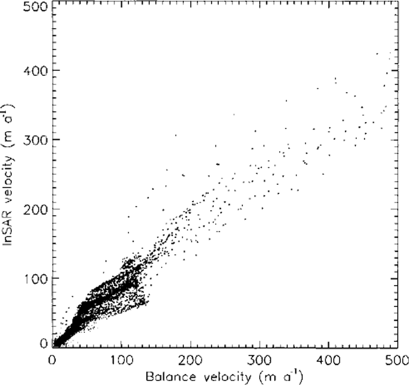
Fig. 2. Balance velocities (Ub) plotted against the InSAR-denved velocities (Uinsar).
The correlation coefficient of the fit was 0.946 and the standard error in Uinsar was ±9.8 m a"1. There is an excellent correlation between the two measurements, although it is evident that Ub has a positive bias with respect to Uinsar, The cause of the bias is not clear at present, although the result implies a thickening in the areas compared (indicated by the yellow polygons in Fig. 1). Ub was also compared with nine global-positioning-system (GPS) measurements over the ice sheet which gave a mean difference of 1.0 m a"1 ±4.4 m a"1 for a mean velocity of 30 m a"1 or in percentage terms 3.6 ±16% (Reference Bamber, Hardy and JoughinBamber and others, in press). Consequently, we believe that, inland, Ub provides a reliable measure of the dynamics, suitable for validating and/or constraining a numerical model.
3. The Thermomechanical Ice-Sheet Model
The numerical ice-sheet model is a fully coupled thermomechanical model that includes basal sliding when the basal ice reaches the pressure-melting point (Reference Huybrechts, Letréguilly and ReehHuybrechts and others, 1991; Reference HuybrechtsHuybrechts, 1996). In this application of the model, all the simulations consider the locally defined depth-averaged velocity for a fixed geometry ("dynamics velocity", Ud), with a steady-state temperature field. The vertical velocities were also derived assuming a fixed geometry. The set-up of the model has been described in detail elsewhere (Reference Huybrechts, Letréguilly and ReehHuybrechts and others, 1991; Reference HuybrechtsHuybrechts, 1996).
Four experiments were undertaken with progressively greater physical processes being incorporated and, therefore, hopefully increasing "realism":
-
(1) isothermal ice, no basal sliding;
-
(2) isothermal ice, with basal sliding;
-
(3) temperature-dependent rheology, no basal sliding; and
-
(4) temperature-dependent rheology, with basal sliding.
For the isothermal experiments, the ice temperature was held at –8°C to produce roughly the same average rate factor as for the temperature-dependent cases. The numerical model simulations were computed at 20 km resolution, and the output of the four runs is shown in Figure 3. To aid comparison, the scaling is the same as in Figure 1 (0–500 m a"1). A direct comparison is, however, not necessarily very meaningful (as discussed later) as Ud can be scaled by a factor of between about 0.1 and 10 (representing the uncertainty in the in-situ ice viscosity). It is, therefore, more useful to plot the ratio or difference of the different velocities. Figure 4 is a plot of the normalized difference between the two velocities: (Ub - Ud/Ub + Ud). Thus values greater than zero represent areas where Ub is larger than Ud and vice versa. The background colour is the value for perfect agreement (a ratio of zero). A value of ±0.333 indicates one velocity is a factor two greater than the other, ±0.5 is a factor 3 and 0.6666 is a factor 5 different. White regions in Figure 4 are areas where there is relatively close agreement.
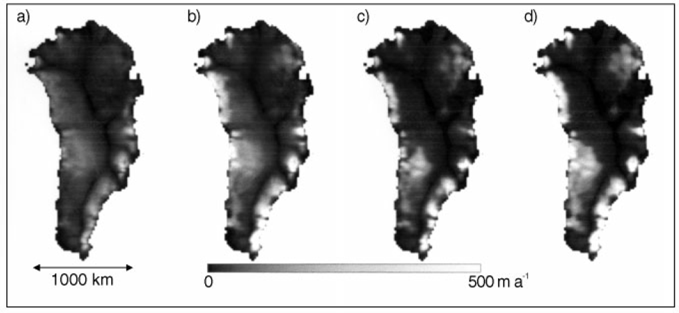
Fig. 3. Dynamics velocities ( Ud) computed using the thermomechanical model for the four simulations: (a) isothermal, no sliding; (b) isothermal with sliding; ( c) thermodynamics included, no sliding: and (d) thermodynamics included, with sliding The scaling is the same as in Figure 1.
4. Discussion
The general pattern of flow shown in Figure 3a–d is as expected as the driving force is surface slope: a common boundary condition. The detail, however, is quite different. For example, the large (>300km) ice stream in the northeast is not generated by the numerical model and much of the detailed flow pattern is completely lost due to the low model resolution (20 km) or perhaps its inherent inability to resolve flow at the sub-gridscale or the fact that longitudinal stresses are not included.
Near the margins, Ub is generally greater than Ud (light grey to white) even for the cases where basal sliding is included (experiments 2 and 4). In the isothermal cases (experiments 1 and 2), Ud generally decreases with respect to Ub moving out towards the margins. This means the ice in the model is too stiff inland and too soft downstream. The introduction of thermodynamics in experiments 3 and 4 appears to partially remove this effect and the agreement in central Greenland is relatively good, suggesting that the ice rheology and thermodynamics (which are coupled) have been reasonably well-prescribed for the summit region and northern sector. It is important to note that the ice viscosity changes by three orders of magnitude from the ice surface to the bed and that, as a consequence of uncertainties in its in-situ value, it is legitimate to scale Ud by up to a factor 2 to obtain better agreement. Thus a uniform shading across each image in Figure 4 implies a good correlation, requiring a uniform scaling factor to be applied. It is evident that this cannot be done for any of the simulations and, as discussed below, the correlation between Ub and Ud does not exceed 0.194 for any of the four experiments. Interestingly, the incorporation of thermodynamics into experiments 3 and 4 appears to create a slight difference between the northern and southern halves of the ice sheet with the model generally underestimating velocities, especially toward the margins, for northern Greenland (ice too stiff) and overestimating them for the southern half (ice too soft). There is, in general, relatively poor agreement near the margins and it is not clear, at this stage, if this is due to inaccurate modelling of the thermodynamics, a flawed relationship between ice rheology and temperature or possibly substantial errors in ice thickness. The overestimation of velocities on the southeastern coast does not appear to be due to basal sliding in the model as Ud is too high in all the runs including the non-sliding cases (1 and 3). In this area the ice appears to be too soft in the model in all the experiments. On the western side from about 72–80° N the converse is the case when the thermodynamics are incorporated (the lighter bands in Fig. 4c and d) suggesting that the modelled temperatures in this region are too cold. The V-shaped light area starting near the centre of the ice sheet and going toward the northeast coast is due to two regions of rapid flow that can be clearly seen in Figure 1. The northern "fork" is the northeast ice stream previously identified in SAR imagery (Reference Fahnestock, Bindschadler, Kwok and JezekFahnestock and others, 1993).

Fig. 4. Normalized difference plot of the balance velocities (Uh) minus the dynamics velocities (Ud) for the four simulations shown in Figure 3.
Figure 5 is a plot of areas of basal melting produced by the model, indicating those areas where sliding can take place. It can be seen that there is an area of basal melt which incorporates much of the northeast ice stream. However, neither experiments incorporating sliding (2 and 4) adequately reproduce this feature although they do show a general improvement in the agreement between Ub and Ud compared with the non-sliding cases in this region. This is most noticeable when comparing experiments 1 and 2 (Fig. 4a and b). The region of large positive differences (i.e. Ub > Ud) is both narrower and shorter in Figure 4b. The southern "fork" (which is less pronounced in Fig. 1) mainly feeds into Waltershausen Gletscher. Figure 5 indicates that no basal melting is produced in this region so the incorporation of sliding makes no difference here. The inclusion of thermodynamics, however, significantly reduces the agreement for this flow feature.

Fig. 5. Areas of basal melting (shaded grey) predicted by the numerical model for simulation 4 (thermodynamics and basal sliding).
At present, only a qualitative comparison has been undertaken. To obtain a more profound understanding of the cause of the differences, it will be necessary to carry out an inverse-modelling experiment, where the balance velocities are used to determine what the ice viscosity and/or thermodynamics must be to reproduce the spatial pattern of Ub. To do this, however, will require improvements in the ice-thickness grid, particularly near the margins (as this directly affects the accuracy of Ub).
The output of the numerical model has also been compared with £/insar and the results of this comparison, for the four experiments, are shown in Figure 6. There is no obvious pattern that can be seen although the inclusion of thermodynamics does seem to produce a slight bi-modal distribution (Fig. 6c and d). The correlation coefficients between the InSAR and modelled velocities are all low, with the highest value being obtained for experiment 2 (τ2 = 0.195).
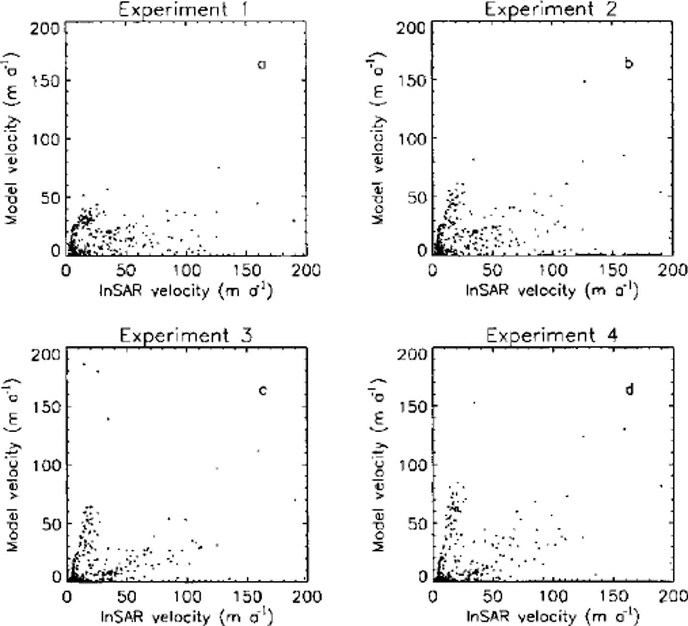
Fig. 6. InSAR-denved velocities (Uinsar) plotted against the model velocities (Ud) for the four experiments described in the text.
A similar picture emerges when Ub is plotted against Ud. Figure 4 shows the spatial pattern of differences, but does not provide an adequate picture of the overall correlation between the two datasets. This is presented in graphical form in Figure 7. As with the comparison with the InSAR data, the correlations are low with the highest value, in this case, being for experiment 4 (r2 = 0.194). As with the In-SAR comparison, the inclusion of thermodynamics produces a slightly bi-modal distribution which we believe is related to the north-south differences discussed above. Due to the large uncertainty in the form of the sliding law and the in-situ viscosity of the ice the agreement between Ub and Ud is almost equally poor for all four experiments and it is, therefore, difficult to conclude, at this stage whether the addition of further physics into the model (in the form of thermodynamics and basal sliding) actually improves the "realism" of the simulated velocity field. With better constraints on the sliding law and in-situ rheology this uncertainty will be removed.
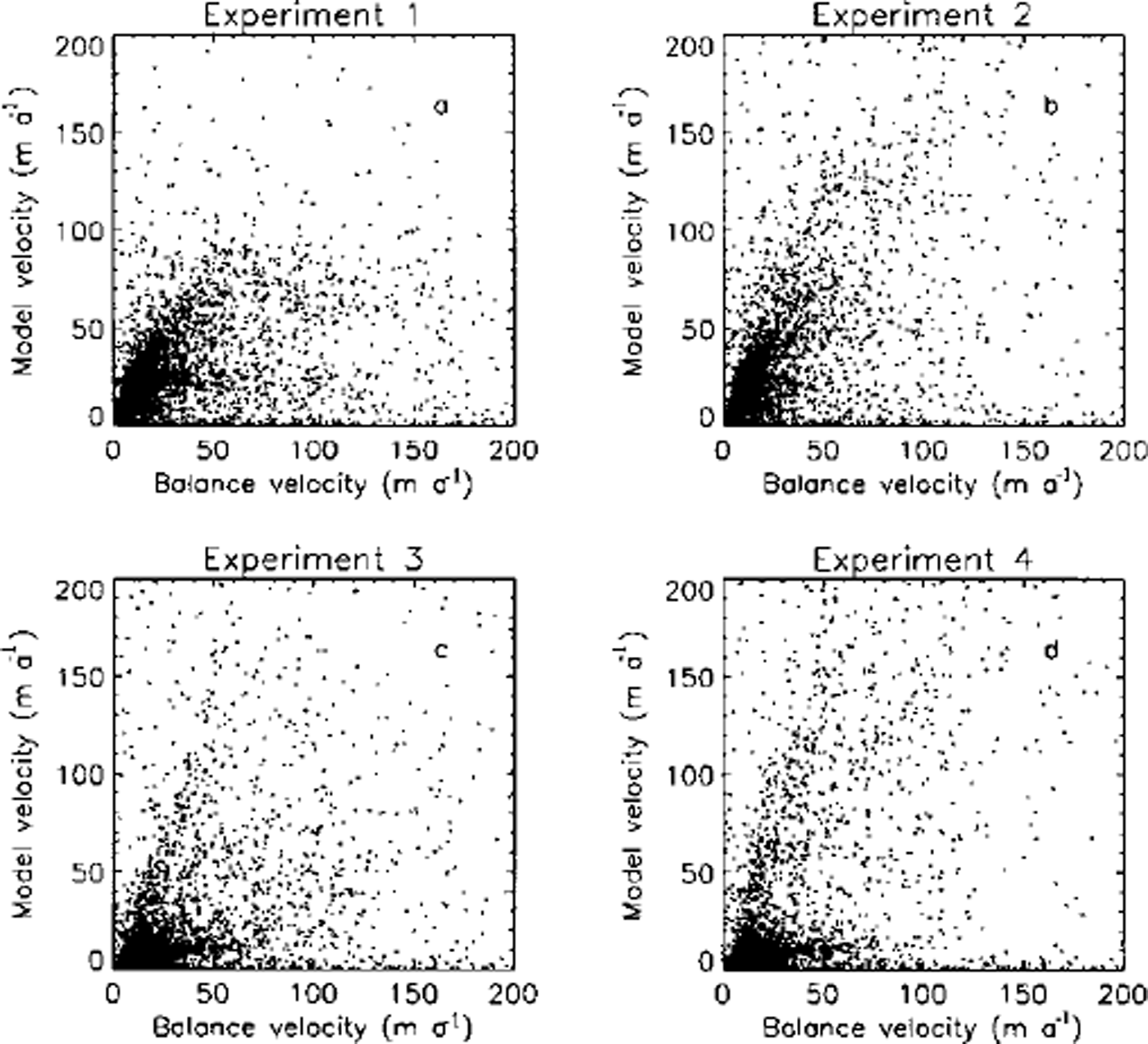
Fig. 7. Balance velocities (Ub) plotted against the model velocities (Ud) for the four experiments described in the text.
5. Conclusions
Balance velocities have been calculated for the Greenland ice sheet using a two-dimensional finite-difference scheme and two new input datasets. These velocities have been compared with surface-velocity measurements derived from SAR interferometry and GPS data. These comparisons have provided confidence in both the computational scheme and the datasets used inland from the margins. The "validated" balance velocities and SAR interferometry have been used to examine the behaviour of a three-dimensional fully coupled thermomechanical model which includes basal sliding, but not longitudinal stresses. Large differences in both the pattern and magnitude of the velocity field were found. The latter, it is believed, is partly due to the uncertainty in the in-situ viscosity of the ice. The former is due, we believe, to the inability of the model to reproduce flow at the grid to sub-grid scale. Ice streams and outlet glaciers, that drain most of the ice from the interior, are very poorly represented in the model due to its resolution and the physics being limited by the use of the shallow-ice approximation and the uncertainty in basal friction when basal melting is generated in the model. The short-term response of the GrIS to global warming appears to be dominated by the surface balance, but it is apparent that the use of models, such as the one presented here, as a tool for predicting the dynamic response of the GrIS to global warming, is questionable.


