2.1. The ice-sheet model

The ice-sheet model treats only grounded ice. Simplifications in the stress-equilibrium equations are made in accord with the so-called shallow-ice approximation (see e.g. Hotter, 1983). Ice flow is assumed to result both from internal deformation and sliding over the bed, which is assumed to be of Weertman type and is restricted to areas which are within 1°C of the pressure-melting point. The rate factor in Glen’s flow law with exponent n = 3 depends on the ice temperature according to an Arrhenitts relation and includes an enhancement factor which depends on the age of the ice. Wisconsin ice (age > 11 500 years) is taken to deform three times taster than Holocene ice, using a method of finding the ire-age boundary as described in Huybrechts (1994). The model has a free interaction between the climatic input and the ice-sheet geometry, which can expand on to the shallow continental shelf in response to lower global sea-level stands. The latter variations control the coastline, beyond which all ice is lost by calving. Bedrock adjustments are incorporated with a two-layer isostasy model, in which the lithosphere depression follows from the local hydrostatic equilibrium and the asthenosphere responds in a damped fashion with a characteristic time-scale of 3000 years.

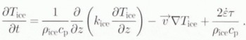
This type of three-dimensional model, similar to other Greenland models developed more recently by other groups (Calov, 1994; Greve and Hutter, 1995; Fabre and others, 1995), has been described in detail elsewhere (Huybrechts and others, 1991; Huybrechts, 1992, 1994), so that the complete set of governing equations does not need to be repealed here. As the focus is on the temperature distribution, however, a short listing of the relevant model equations and their boundary conditions is appropriate:Ice temperature:

(1)

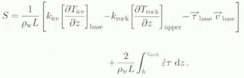
Bed temperature:

(2)

Basal-melting rate:

(3)

Ice–rock boundary condition:

(4)

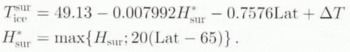
Ice–atmosphere boundary condition:

(5)

Lithosphere lower boundary condition:

(6)

In the above equations, T is temperature (°C), t is time (a), and τ are the effective strain rate (a⁻¹) and effective deviatoric stress (Pa) in the formulation of the strain heating, H is ice thickness (m), h is bed elevation (m), H _sur is surface elevation (m), Lat is geographical latitude (°N), ∆T is temperature forcing (°C), S is the melting rate (ma⁻¹), τ _base is basal traction (Pa), υ is velocity (ma⁻¹) and G is geothermal heat flux (Wm⁻²). The other physical parameters are listed in Table 1. z _melt is the upper boundary of a temperate basal layer, which may eventually develop in the calculations and which assumes that all produced meltwater is drained away at the base. Apart from that, there is no further treatment of such a temperate ice layer, if any, or its surface boundary with the cold ice, and T _ice in Equation (1) is simply replaced with T _melt whenever the latter is reached. Other simplifications made in Equation (1) include the use of a constant density in the firn layer and the neglect of horizontal heat conduction, which is acceptable on the scales considered.

2.2. Numerical features

All equations are solved on a grid by the finite-difference method. The horizontal grid size is 20 km and there are 26 layers in the vertical, with a closer spacing near the base where the shear concentrates. Rock temperatures are calculated down to a depth of 2 km in time-dependent situations, with a total of six points which are equally spaced 400 m apart. This depth appears to be sufficient to capture most of the effect of temperature variations operating on the glacial–interglacial time-scale (Ritz, 1987; Huybrechts, 1992). For the thermal diffusivity of the bedrock adopted in this paper, a rock depth of 2 km will attenuate 99% of the amplitude of a wave with a period of 20 ka and 87% of the amplitude of a wave with period 100 ka (e.g. Paterson, 1994, p. 206–207).

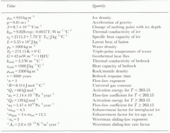
Table 1. The physical parameters used in the madel and the parameters used in the flow law (*) and the basal sliding relation (^†) are included for completeness and comparison with other work (Huybrechts and others, 1991)

All spatial differences are of second-order accuracy, including the upstream differences required to deal with the advection terms. Oilier features include an Alternating Direction Implicit (ADI) method for solving the height-evolution equation, an implicit scheme in the vertical for the heat-flow equations, and the use of a vertical coordinate which is scaled to local ice thickness. Time steps are 2.5 years for ihc ice-thickness calculations and 50 years for the temperature calculations. The model runs on a CRAY C90 and takes about 1.3 h of CPU time for a 100 000 year integration.

2.3. The mass-balance treatment

The surface mass-balance components are snow accumulation and meltwater run-off, both of which are parameterized in terms of temperature. The forcing consists of a background temperature change ΔΤ, which is uniformly distributed over the ice sheet and throughout the year.

As in previous studies with earlier versions of the model, the presently observed precipitation rate is taken as a base (from Ohmura and Reeh, 1991) and prescribed to vary by a factor (1 + s) for every degree of change in mean annual air temperature ∆T, so that

where

(7)

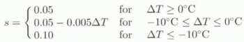
and Pree(t) and Prec(0) are precipitation rates (in m a⁻¹ of ice equivalent) at time t and at the present time, respectively. The temperature-dependence of the factor (1 + s) is a refinement with respect to previous studies. It combines the change in precipitation rate per degree Celsius of 5.33% found by Clausen and others (1988) from shallow ice cores spanning the late Holocene with the 8–9% value derived by Dahl-Jensen and others (1993) for the upper 2321 m of the GRIP core. The relation adopted in Equation (7) is also in better agreement with accumulation studies conducted on the GISP2 core (Kapsner and others, 1995). For a temperature lowering of 5°C, precipitation rates are reduced by 30.3%, and for a cooling of 10°C, they are reduced to 61.4%.

Unlike the parameterization proposed by Fabre and others (1995), Equation (7) does not include the potential effects of changes in the local surface slope as there are little or no data to substantiate such a relation. Nevertheless, the neglect of changing precipitation patterns, especially in situations where the ice sheet significantly changes its geometry, remains a major simplification in the accumulation treatment adopted here.

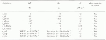
Table 2. Overview of the forcing applied in the various model experiments. Experiments beginning with “s” are Steady states, those beginning with “c” are glacial cycle runs. ∆T is the background temperature forcing, H _sl is the sea-level forcing, G is the geothermal heat flux, and a and b are parameters to convert δ ¹⁸ O data to a temperature forcing (Equation (8)) or a sea-level forcing (Equation (9)), respectively. ^# , temperature only forces the surface temperature; ^† , temperature only forces the mass balance

The mell-and-run-off model is based on the degree-day method and is similar to the model described in Reeh (1991), albeit with a few amendments. In accordance with measurements on glaciers in central West Greenland, degree-day factors were chosen as 3 mm/PDD for snow melting and 8 mm of ice equivalent per positive degree-day for ice melting. The melt model further takes into account the daily temperature cycle and includes a probability function which allows for positive temperatures even when the mean daily temperature is below freezing. Using the same Gaussian probability distribution with a standard deviation, σ, of 5°C, the fraction of precipitation falling as rain is set equal to the probability that the surface air temperature rises above 2°C. The liquid water (meltwater and rain) produced by the model will at first refreeze in the snow-pack and produce superimposed ice. The maximum limit on the production of superimposed ice is set equal to the latent-heat release needed to raise the uppermost 2 m of the ice sheet from the mean annual temperature to the melting point. This value gives a good fit to a number of detailed measurements reported by Ambach (1963). The resulting surface warming also contributes to the surface-boundary condition for the temperature of the ice sheet (Huybrechls and others, 1991).

2.4. Model forcing during glacial cycles

In the glacial cycle runs, the mass-balance and surface-temperature relations were forced by the GRIP δ ¹⁸O record at a 100 year resolution (Dansgaard and others, 1993). This record was taken to span entirely the last two glacial cycles starling at 225 000 years ago. The δ ¹⁸O (in ‰) values were converted into background temperature changes ∆T according to

(8)

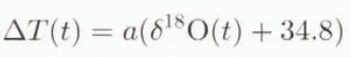
where a = 1.5°C‰⁻¹ is the standard value for the δT ¹⁸O conversion ractor (Johnson and others, 1989). This parameter will, however, be allowed to vary in the experiments described later.

The sea-levet forcing ∆H _sl (m) was derived from the Specmap stack (Imbrie and others, 1984) over the same lime period according to

(9)

where δ ¹⁸O_m (in ‰) are marine oxygen-isotope values and n = −34.83 m ‰⁻¹. This forcing was made to start off with a zero sea-level change at 225 ka BP and reaches a maximum sea-level depression of 130 m at 19ka BP. Between 4ka BP and the present time. ∆H _sl was set to zero.

3. The Resulting Temperature Conditions

Two series of model runs were aimed at investigating Steady-State and time-dependent conditions, respectively. The forcing applied in these model experiments is specified in Table 2, with a summary of several large-scale characteristics given in Table 3.

3.1. The interglacial experiment

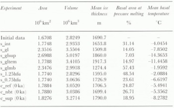
The interglacial reference run was defined by starting from the observed ice-thickness and bedrock data (Letréguilly and others, 1991a), and integrating the model to steady state with a zero-temperature perturbation (ΔT = 0 in Equation (5) and (7)) and standard values for physical parameters (table 1). The initial englacial temperature distribution was linear with a gradient of −6.5°C per 1000 m, This run (s_int) did not include heat conduction in the bedrock and was made over 300 000 years to approximate unquestionably the stationary state. The values listed in Table 3 indicate that the modelled area and volume are then within a few percent of the initial data. This is acceptable, as it is not exactly known how far the present ice sheet is out of steady stale.

Table 3. Summary of the main experimental results for the model runs described in Table 2. The values for area and volume use a constant grid-cell area of 20 km × 20 km and have not been corrected for distortions due to the map projection (polar stereographic with standard parallel at 71°N). These vary from −2.0% at 80° N to + 4.2% at 50°.N

The corresponding basal-temperature field is displayed in Figure 1. It can be seen that temperate ice, which accounts for about 31% of the total basal ice-sheel area, is mainly confined to the coastal region and in a number of fast-flowing outlet glaciers. Only in the central western area and in the northeast of the ice sheet does temperate ice extend farther inland. Most of the central ice sheel has homologous basal temperatures of between 6° and 10°C below the pressure-melting point. Colder ice is mainly situated in regions with thin ice in the cast and in a number of zones in the northwestern quadrant. Here, local ice divides form perpendicular to the ice-sheet margin which are characterized by low flow velocities and dissipation rates.

These temperatures generally agree within 1–2deg with a similar map presented in Greve and Hutter (1995). The reasons for these (albeit small) differences are unclear. Possible causes may include variations in climatic input and flow-law parameters, their higher vertical resolution or specific handling of temperate ice layers near the base, or alternatively, from the longer integration times, the inclusion of bedrock adjustment or the higher horizontal resolution used in this study. On the other hand, our result is quite different from the basal temperature map obtained by Calov (1994) for a fixed ice thickness. That is because the assumption of a fixed geometry results in a diffent internal velocity distribution and, consequently, a different advective contribution in the beat equation.

3.2. Steady-state sensitivity experiments

The main series of steady-stale experiments considered shifts in environmental conditions of typical glacial–interglacial magnitude. These are a temperature towering of 10°C, the associated lower mass-balance conditions and a sea-level depression of 130 m, either singty or in combination (cf. Table 2). To assess fully the effects of glacial-boundarv conditions within their uncertainties, a super-glacial experiment was also conducted (s_glsup), in which the temperature was lowered by 20°C, the ice sheet was allowed to expand to the −260 m isobath and the parameter ‘s’ in Equation (7) was halved to remain in accordance with the δ ¹⁸O/ accumulation gradients derived from ice cores. Such an experiment reflects the uncertainty in the conversion factor from oxygen-isotope ratio to temperature in the Greenland ice-core records (personal communication from S. J. Johnson), which may amount to twice the commonly used value of 1.5°C‰⁻¹ (Equation (8)), and hence, imply a Wiseonsin–Holocene temperature shift of around 20°C (Cuffey and others, 1995).

Typically, steady-state “glacial” conditions (s_gl) produce a mean cooling at the base of about 3–4°C, which is only a fraction of the applied surface cooling of about 10°C. This is in large part because of the counteracting effect of the reduced accumulation rates, which result in less advection of cold ice born above, and hence in a warming. In addition, there are effects due to thermal diffusion (thicker ice increases the insulating effect of the ice and makes the evacuation of the geothermal heat to the surface more difficult), heat dissipation and the dependence of the thermal parameters on temperature, all to different degrees at different places (Ritz, 1987; Hindmarsh and others, 1989; Huybrechts, 1992).

The effects on the temperature field of mass-balance and surface-temperature dinners are nicely demonstrated in two other runs. In an experiment where only the surface temperature is lowered (s_gltem), the applied cooling is transferred to the base almost unchanged, indicating that the combined changes in advection, dissipation and conduction are small. In another where only the accumulation rates are reduced (s_glmb), an almost continuous area of temperate ice occurs over nearly 60% of the basal area. Here, the warming effect of the lower accumulation rates is much stronger than the cooling effect of the decreased frictional heating, especially in central areas. This is in stark contrast to the superglacial run (s_glsup), where almost all of the base is frozen to bedrock, except at the nutlet glaciers where sufficient dissipative heat can still be generated.

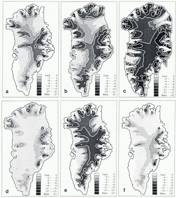
Fig. 1. A comparison of steady-state temperature fields under various forcings as detailed in Table 2. Temperatures are shown in °C below the pressure-melting point. The lightest shading showi ice at the pressure-melting point, the darkest shading is for ice at the lowest temperatures. a, Interglacial reference run (s_int); b, Standard glacial run (s_gl); c, Superglacial run (s_glsup); d, Glacial mass-balance effect only (s_glmb); e, Glacial temperature effect only (s_gltem); f, 125% geothermal heat flux (s_1.25hfu).

For the purpose of comparison, two additional interglacial runs were performed to illuminate the uncertainties in the value of the geothefmal heat flux G; one run is also displayed in Figure 1. In these experiments, G was respectively raised to 125% (s_1.25hfu) and lowered to 75% (s_0.75hfu) of its standard value of 1 HFU, which is considerably less than the observed variations of this quantity. Clearly, increasing the basal-heat input increases the area of pressure melting, while lowering it decreases it. The effect of a ±25% change in the geothermal heat flux on the melt area is nearly of the same order as a glacila–interglacial shift, However, although the value of G is certainly important for a diagnosis of the present state, this does not necessarily have to mean that the sensitivity of the basal-temperature field to external climatic forcing is equally affected. Further experiments revealed that basal-temperature differences at a specific location between, for example, runs s_int and s_gl, only weakly depended (< 5% difference) on the exact value of the geothermal heat flux, while G ranged between 0.75 and 1.25 HFU and basal temperatures remained below the pressure-melting point. The implication is that differences of basal temperature as produced by the model are not necessarily in error even when their absolute values deviate from reality. It also means that, given the basal temperature, the model can be used to predict G, which could then be further verified against the vertical temperature profile obtained in boreholes.

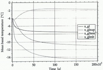
Fig. 2. Evolution of the mean basal temperature after a glacial–interglacial step change in environmental boundary conditions. These curves demonstrate the very long response time-scales needed to approximate a new steady state (s_gl = standard glacial run, S_glsup = super glacial run, s_gllem = glacial temperature effect only s_glmb = glacial mass-balance effect only). In these runs, heat conduction in the bedrock below was not considered.

The corresponding ice-thickness distributions are not shown here but are summarized in Table 3. All experiments which only involve temperature changes (s_gltem, s_1.25hfu, s_0.75hlu) did not produce recognizable changes of the ice-sheet extent, though the local ice thickness is affected. These thickness changes are inversely related to temperature at the base; the colder the ice, the less readily the ice deforms, leading to decreased strain rates and ultimately a thickening. The effect is certainly not negligible and typically amounts to about 1.5% change of ice thickness for every degree of basal-temperature change. In addition, there is the effect on ice thickness from basal sliding as the latter is coupled to basal temperature. Changes in the lateral extent, on the other hand, are controlled by changes of the surface mass balance and by the prescribed coastline. In those experiments, local ice thickness is also a function of the ice-sheet span and of the mass balance. For the glacial experiment, s_gl, for instance, the end effect is an ice sheet whose area and ice volume are larger by 32 and 21%, respectively, though the mean ice thickness is 9% lower. All these results demonstrate that, in order to study adequately ice-thickness changes in response to external forcing, one has to take into account the mutual coupling between ice flow and ice temperature. That is, because changes in the surface climate not only alter the ice-sheet’s mass balance but also its thermal regime, which affects the flow properties of the ice.

3.3. Time-dependent experiments

The results just described assume an ice sheet in steady state. In reality, however, it is unlikely that such a state would ever be reached, because climate varies on a substantially shorter time-scale than the response time-scales associated with thermomechanical coupling. This is demonstrated in Figure 2, which shows how basal temperatures respond to a stepwise change in boundary conditions. The slowest component within the system is heat conduction (s_gltem) and the resulting curve clearly indicates that it may lake up to 100 150 ka before a new stationary stale is established.

To evaluate the consequences for the Greenland ice sheet, three time-dependent experiments were carried out simulating the last two glacial cycles (table 2), including a superglacial cycle experiment (c_sup) using a conversion factor of 3°C‰⁻¹ (a in Equation (8)) together with the associated halved precipitation parameters “s” in Equation (7). In the latter experiment, positive temperature perturbations, in particular during the Eemian interglacial when GRIP δ ¹⁸O values increase to as much as −31.5‰, were clamped according to ΔT(t)* = ΔT(t) (0.5 + 0.5 exp(−0.125ΔT(t))). This prevents the ice sheet from melting entirely, which would be in contradiction with the very existence of the GRIP record itself. That such damping should be needed indicates that the assumptions made in the c_sup experiment may not be valid for warmer climates. This, however, is of little significance for the present study. The c_sup experiment also considered a doubled Specmap sea-level forcing. All of these experiments were cycled over three identical periods of 225 000 years to ensure that the model had entirely forgotten its initial set-up conditions.

Figure 3 compares temperature shifts at the base since the Last Glacial Maximum at 18 ka BP for the standard cycle experiment (c_ref) with the model’s interglacial (s_int) and glacial (s_gl) steady states. Clearly, the temperature response is strongly damped during a glacial cycle. At 18 ka BP (panel a), temperatures below the central dome were near their steady-state values, though marginal temperatures were still warmer by 2–3°C. Between 18 ka BP and the present time (panel b), the basal-temperature rise exhibits a near concentric pattern from near-zero values in the centre to values up to 6°C near to the margin. This pattern reflects the variation in basal-temperature reaction times, which are longest at the base in the centre, where heat transfer by advection is slower. It is shortest at the margin because of higher ice turn-over rates and because increased dissipation has an immediate effect on basal temperature. As shown in panel c, bottom temperatures are still out of balance with the present-day climate by typically 3–4°C, except for those areas which have always been at the pressure-melting point.

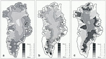
Fig. 3. Basal-temperature differences (°C) between different time intervals for the standard cycle experiment (c_ref). a, Difference between the glacial state (s_gl) and 18 ka BP(c_ref); b, Difference between 18 ka BP (c_ref) and present (c_ref); c, Difference between the present (c_ref) and the interglacial reference run (s_int). The corresponding fields for the supercycle experiment (c_sup) has values between 50 and 100% higher but similar patterns.

The corresponding evolution of mean basal temperature and the percentage of the base at pressure melting are shown in figures 4 and 5. These curves should be compared with the associated glacial and interglacial stationary states which would occur if the climate were stable for a sufficiently long time. Apart from re-affirming the damped response slated above, this brings to light that basal-temperature conditions have generally been nearer to glacial rather than interglacial conditions, which is not surprising as glacial conditions dominated the last 225 000 years of the climatic history. Excluding the thermal response of the bedrock (c_nbt) causes the total basal temperature range during a glacial cycle to increase by about one-third. This means that the effect of heat conduction in the bedrock cannot be neglected during a glacial cycle.

Fig. 4. Evolution of the mean basal temperature of the ice sheet during the last two glacial cycles for the experiments c_ref (standard glacial cycle run). c_sup (super glacial cycle run) and c_nbt (standard glacial cycle without heat conduction in the bedrock).

Fig. 5. Percentage ice-covered basal area which is at the pressure-melting paint for the standard cycle experiment (c_ref) and the supercycle experiment (c_sup). For bath experiments, the fraction at melting point never exceeds the fraction frozen to the bedrock.

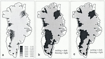
Fig. 6. Three plots addressing various aspects of basal melting during and after the last two glacial cycles. Panel (a) shows the basal-melting rate predicted by the model for the standard cycle experiment at present (c_ref). The dark shading panels (b) and (c) indicate where basal melting has occurred at some time during the past 225000 years in the standard cycle experiment (c_ref; panel (b)) and the supercycle experiment (c_sup; panel (c)).

The spatial pattern of basal melting during the last two glacial cycles is shown in figure 6. The area of basal melting has always been confined to the northeastern and southern parts of the ice sheet and has never exceeded the area at basal freezing. Melting at the base in a few places presently frozen to bedrock occurred during the Eemian and is due to the retreat of a temperate margin to locations behind its present extent (cf. Letréguilly and others, 1991b). The present basal-melting rate as calculated with Equation (3) peaks at up to 10 cm a⁻¹, but it usually remains below 1 cm a⁻¹. The corresponding basal-temperature field for present conditions in the c_re(experiment is not shown but it can be calculated In subtracting values in Figure 3 (panel c) from those in Figure 1 (s_int) for those areas not presently at pressure melting as shown in Figure 6 (panel a).

4. Comparison With ICE Cores

It is difficult to compare the complete temperature results with reality, because the basal-temperature field has only been measured in a few deep boreholes. Table 4 Summarizes the model results at grid points nearest to the deep-drilling sites of Camp Century, Dye 3 and Summit (GRIP). These grid points are at most 14 km away from the exact borehole locations, which is roughly the mapping error in the original ETOPO5 and radio-echo-sounding data (Leiréguilly and others, 1991b). In the steady state, modelled bottom temperatures are within 1–2°C of the observations for Summit and Camp Century, which is surprisingly close, but differ by almost 9°C for Dye 3, for which there is no straightforward explanation, In the cycle runs c_ref and c_sup, on the other hand, basal temperatures at the present time are significantly colder than the measurements by between 2° and 6°C. These are the temperatures which should be compared with the observations.

There are many possible explanations for the mismatches between modelled and observed temperatures. One explanation is errors in the input data. The modelled ice thicknesses, for instance, deviate from reality by typically 100 m, which is about the accuracy of the geometric input data (Letréguilly and others, 1991a). There are also slight deviations in the gridded accumulation data as compared to the borehole values. Another explanation could be deficiencies in the ice-sheet model. The shallow-ice approximation is known to be less accurate at domes and the model does not deal with stress-induced anisotropies, which could have a significant effect on the basal temperature field. Also, one can select many sets of values for the climatic history (surface temperature and mass balance), the geothermal heat flux, or to a lesser extent, for the formulation of the ice flow (flow-law, enhancement factor, basal sliding), which would give a better fit. For instance, some further experimentation showed that basal temperatures could be exactly matched by varying the geothermal heat flux within about 50% of its standard value, while keeping everything else equal. These heat fluxes (in HFU) were for experiment c_ref: Camp Century: 1.21; Dye 3: 0.44; Summit: 1.17, and for c_sup: Camp Century: 1.59; Dye 3: 0.68; Summit: 1.50, all of which ate within the expected range of uncertainty for this quantity (1HFU = 42 mW m⁻²).

Table 4. Summary of results for grid points nearest to the deep ice-core-drilling sites of Dye 3, Camp Century and Summit for the experiments described in Table 2. H is ice thickness, T _bas is basal temperature and M is the mass balance. An asterisk denotes a temperature at the pressure-melting point.

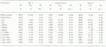
Fig. 7. Evolution of basal temperature in locations close to the boreholes of Camp Century, Dye 3 and Summit for a standard geothermal heat flux of 1 HFU (42 mW m ⁻² ). The upper curve of each pair is for the standard cycle experiment (c_ref) and the lower curve is for the supercycle experiment (c_sup). Zero temperatures at Dye 3 around 125 ka <SC>BP> are because this location is no longer ice-covered during the warmest part of the Eemian interglacial.

These changes did am appreciably affect the magnitude of the response during the evolution experiment and produced only linear shifts with respect in the ordinate in the curves shown in Figure 7. These curves suggest that, during the last 225 000 years, basal melting never took place at Camp Century and Summit, indicating that basal ice was not lost, Dye 3, on the other hand, would according to these calculations have experienced basal melting shortly before and after the time when this location became ice-free during the Eemian.

5. Conclusions

The temperature fields discussed in this paper indicate that most of the base of the Greenland ice sheet is frozen to bedrock. Pressure melting is mainly confined to the coastal margin and the northeastern and central western parts of the ice sheet, and it has been during the last two glacial cycles. The results, assuming steady state, exhibit a large sensitivity to glacial–interglacial shifts in surface-boundary conditions. However, in non-steady-state glacial cycle simulations, the basal-temperature response is strongly damped, in particular in central areas. Consequently, palaeotemperatures still exist beneath the Greenland ice sheet and bottom temperatures are out of balance with the present-clay climate by typically 3° to 4°C. The implication is that the ice sheet will still be responding to its climatic history for a long time to come, irrespective of future climatic trends.

The basal temperatures produced by the model for standard parameter values were in reasonable agreement with the temperatures measured at Camp Century and Summit but much too warm at Dye 3. The reasons for these discrepancies were not entirely clear. However, basal temperatures were shown to be very sensitive to the value of the geothermal heat flux, which is poorly constrained and likely to vary from one region to another. A ±25% change in the geothermal heat flux produced nearly the same temperature difference as a typical glacial–interglacial contrast, though the sensitivity of the basal temperature field to external climatic forcing was little affected by the exact value assumed for the geothermal heat flux. Because of such deviations of the model from reality, due to uncertainties in the input data and the interactions among the model variables, these large-scale three-dimensional calculations seem best suited for determining changes with respect to a reference state rather than absolute values.