


1. Introduction
In this paper, we apply the avalanche dynamics program RAMMS (Rapid Mass Movements) to model the In den Arelen avalanche event. This avalanche occurred near Davos, Switzerland, in the early morning of 27 January 1968, striking a farmhouse and killing four inhabitants (Fig. 1). Because of the extreme run-out distance, the In den Arelen event was instrumental in determining extreme run-out friction parameters of the Voellmy–Salm avalanche dynamics model (Reference Salm, Burkard and GublerSalm and others, 1990). It is a well-documented event (SLF, 1969) and aerial photographs from 1956 show the extent of the forested terrain (Fig. 2). Snowfall and wind measurements from the Weissfluhjoch research station can be used to estimate release depths and snow-cover entrainment depths. Recently a high-resolution (2 m) digital terrain model of the region has been obtained.
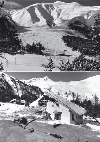
Fig. 1. The In den Arelen avalanche track. Note the long flat runout zone. In the immediate foreground of (a), the overhead power lines of the railway can be seen. The central arm of the avalanche penetrated the forest, destroyed several houses (b) and crossed the railway line (photographs: SLF).
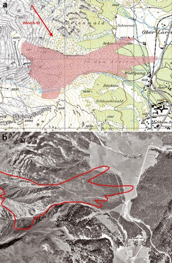
Fig. 2. Documented extent of the In den Arelen avalanche. (a) Wind direction and wind speed are depicted in the upper left-hand corner (map: PK25Q2009 swisstopo (DV033492)). (b) Aerial photograph of the forest cover in 1956 (photograph: SLF).
The In den Arelen avalanche is difficult to simulate with one-dimensional avalanche dynamics models, such as AVAL-1D (Reference Bartelt, Salm and GruberBartelt and others, 1999; Reference Christen, Bartelt and GruberChristen and others, 2002). One-dimensional modelling of this event requires simplifying the complex distribution of release zones, distributing the mass between the different multiple-flow channels and estimating the flow width of the open run-out zone. We therefore apply the two-dimensional avalanche dynamics model RAMMS to demonstrate how advanced engineering models can be used (Reference Christen, Kowalski, Bartelt and StoffelChristen and others, 2008). These models can exploit new computer technology, especially geographic information systems, maps and aerial photograph rendering, as well as three-dimensional terrain visualization. However, many fundamental modelling problems remain (or have become even more difficult), such as the definition of release areas in three-dimensional terrain, assessing the frictional role of terrain and vegetation and, finally, introducing snow-cover entrainment, which greatly affects the overall mass balance of avalanche events. Another issue that demands attention is the appropriate resolution of the digital elevation model (DEM) and the computational model.
2. RAMMS Model Equations
We solve the following system of differential equations for the avalanche flow height, H(x, y, t), velocities, Ux (x, y, t) and Uy (x, y, t), and the kinetic energy associated with the random movements of snow granules, R(x, y, t), at time t, where the topography, Z(X, Y), is given in a Cartesian framework, X and Y being the horizontal coordinates. The surface induces a local coordinate system, x, y, z. It is discretized such that its projection onto the X-Y plane results in a structured mesh. From first principles of mass and momentum conservation, the fundamental balance laws are derived:

![]() in the mass-balance equation (1) denotes the mass production source term, referred to as the snow entrainment rate
in the mass-balance equation (1) denotes the mass production source term, referred to as the snow entrainment rate ![]() or the snow deposition rate
or the snow deposition rate ![]() . The field variables of interest are the avalanche flow height, H(x, y, t), and the mean avalanche velocity,
. The field variables of interest are the avalanche flow height, H(x, y, t), and the mean avalanche velocity, ![]() . The magnitude and direction of the flow velocity are given by
. The magnitude and direction of the flow velocity are given by ![]() and the unit vector
and the unit vector ![]() respectively. The right-hand sides of the momentum equations (2) and (3) sum to the effective acceleration of the avalanche. The terms
respectively. The right-hand sides of the momentum equations (2) and (3) sum to the effective acceleration of the avalanche. The terms
define the gravitational accelerations in the x and y directions, respectively. The acceleration normal to the avalanche slope is given by gz and the active/passive pressure coefficient by k a/p (Reference Bartelt, Salm and GruberBartelt and others, 1999). Frictional decelerations in the x and y directions are given by
and
where μ(R) and ξR) are the Voellmy model friction coefficients (Reference SalmSalm, 1993). Equation (4) denotes the depth-averaged production/decay relation of the fluctuation energy (Reference Buser and BarteltBuser and Bartelt, 2009).
Entrainment is modelled using a rate-controlled approach which allows us to regulate both the mass uptake and the time delay required to accelerate the mass to the avalanche velocity. The effective entrainment rate, ![]() (that is, the entrainment rate at which the mass is moving with the avalanche velocity), is parameterized by the dimensionless entrainment coefficient, κ:
(that is, the entrainment rate at which the mass is moving with the avalanche velocity), is parameterized by the dimensionless entrainment coefficient, κ:
The initial value, hs(x, y, 0), is given by the total height of the snow cover at position (x, y) and time t = 0s. It is given by the sum of the single layer heights hs = Σ hi. In RAMMS we limit the number of snow layers to three: i ∈ {1,2,3}. We assume that the ith snow layer has height hi
, constant entrainment coefficient Ki
and constant snow density ![]() . The snow layers correspond to previous snowfall events. The density of the avalanche is denoted by p. Typically, when Ki > 1, we have near-instantaneous entrainment and densification of the snow cover, although the entrainment rate depends also on avalanche speed. For Ki < 1, snow is entrained into the avalanche, but at a much slower rate. Therefore, different values of κi
correspond to different entrainment mechanisms. For frontal ploughing we have found 1 ≤ κi ≤ 5 and for basal erosion κi ≤ 1.
. The snow layers correspond to previous snowfall events. The density of the avalanche is denoted by p. Typically, when Ki > 1, we have near-instantaneous entrainment and densification of the snow cover, although the entrainment rate depends also on avalanche speed. For Ki < 1, snow is entrained into the avalanche, but at a much slower rate. Therefore, different values of κi
correspond to different entrainment mechanisms. For frontal ploughing we have found 1 ≤ κi ≤ 5 and for basal erosion κi ≤ 1.
The coefficients a and β of Equation (4) define the production and decay of random kinetic energy (Reference Buser and BarteltBuser and Bartelt, 2009). The functional dependency of the Voellmy coefficients on the mean random kinetic energy, R, is explained in detail by Reference Bartelt and BuserBartelt and Buser (2010). Recently, experiments in Vallée de la Sionne, Switzerland, have shown that the Swiss guideline recommendations for extreme μ and ξ values, typically μ = 0.155 and ξ = 3000ms∼2, correspond to high R values found at the front of the avalanche (Christen and others, in press). The Swiss guideline recommendations can, therefore, accurately describe the mobility of the avalanche head and thus correctly reproduce the maximum avalanche velocities, as well as the maximum run-out distance. When a = 0, there is no production of random kinetic energy and the model corresponds to the classical Voellmy model. In this paper, we perform simulations with a = 0, that is, using the Swiss guideline μ and ξ recommendations. Finally, the second-order numerical solution procedure is described by Reference LeVequeLeVeque (2002), Reference Yoon and KangYoon and Kang (2004) and Reference KowalskiKowalski (2008).
3. The In Den Arelen Avalanche
The In den Arelen avalanche track is characterized by multiple release zones and a long, open run-out zone that is partly forested. The 1968 avalanche flowed in three different arms, with varying run-out distances (Fig. 2). The far-reaching central arm destroyed a large amount of forest and struck a farmhouse, transporting the roof ∼150 m before stopping. This arm crossed the Klosters-Davos railway line, running several hundred metres on a flat, partly vegetated slope of 8–12°. The northern arm of the avalanche flowed through forest, stopping near another farmhouse, while the southern arm stopped shortly above Davos Wolfgang. A brief description of the In den Arelen avalanche is given by SLF (1969). More detailed information was found in the SLF archives. This information included local newspaper reports, several photographs of the avalanche run-out zone and a sketch of measured deposition heights (∼2 m; see section 4.4) near the destroyed farmhouse and railway lines. Former SLF researchers B. Salm and O. Buser were contacted, and supplemented the written documentation with eyewitness reports.
3.1. Release zones
RAMMS offers two ways to specify release zones. Firstly, the perimeters of the release area can be specified by hand-drawing polygon shapefiles. This procedure usually requires tracing the release polygons on slope-angle maps, automatically generated within RAMMS from the DEM. Secondly, an implemented Geographical Information System (GIS)-based terrain analysis classifies potential release areas automatically. This analysis considers not only slope angle, but also planar curvature, altitude and vegetation (Reference Maggioni and GruberMaggioni and Gruber, 2003). Automated procedures are required for large-scale hazard-mapping applications with RAMMS (Reference Gruber and BarteltGruber and Bartelt, 2007). The fracture depth in the release zone can be defined individually for each release zone, or automated procedures based on the Swiss guidelines for avalanche calculations (Reference Salm, Burkard and GublerSalm and others, 1990) can be employed. In this case the fracture depth in the starting zone is specified according to the mean slope angle in the release area.
Information concerning the release areas and release depths is sparse, but documentation and eyewitness accounts indicate three release basins. For this reason, the release areas were first identified using the automated procedure (see Fig. 3). The automated procedure found areas that were in agreement with the observations for all three basins. Regions not in agreement with the documented release areas were discarded. Strong winds from the northwest (Fig. 2) and a 3 day snow amount of ∼80 cm were recorded at the nearby SLF Weissfluhjoch research station. This information was used to determine the release depths. On southeast-facing slopes we assumed an additional 45 cm of snow due to snowdrift (release depth on northwest slopes were decreased by 20 cm). Release depths of 0.6–1.25 m were used, resulting in a total starting volume of 175 000 m3.

Fig. 3. (a) Automatically generated potential release areas. (b) The final release areas used for the simulations. Note the three release basins (green, blue and orange areas). Release depths on southeast-facing slopes are higher because of strong northwesterly winds (map: PK25©2009 swisstopo (DV033492)).
3.2. Forest
Eyewitness accounts of the avalanche reported woody debris in the avalanche depositions. The influence of forested terrain is taken into account in RAMMS by adapting the friction parameters, μ and ξ. The μ coefficient is slightly increased, by 0.05, while the velocity-dependent ξ coefficient is significantly reduced, typically to values ξ = 400 m s – 2. The location and extent of forest stands are defined by polygon shapefiles or by grids with 0 (for no forest) or 1 (for forest). For the In den Arelen case study, we overlaid aerial photographs of the region and defined polygon shapefiles by tracing the forested areas. We did not specify forest in the primary flow direction of the central flow arm, since we assumed this forest stand was easily destroyed and did not decelerate the avalanche. This procedure is common practice in Switzerland and is based on the idea that the energy consumed by breaking or overturning trees is small in comparison to the overall kinetic energy of the avalanche (Reference Bartelt and StöckliBartelt and Stöckli, 2001).
4. RAMMS Simulations
4.1. Release zones, avalanche volume and snow-cover entrainment
Scenarios
The avalanche naturally released during the night, so no information is available about whether all the release areas released together or whether the zones released individually. We therefore computed three different scenarios: (1) all three zones released spontaneously at the same time; (2) each zone released individually starting from the north and moving south; and (3) each zone released individually starting from the south and moving north. In RAMMS the avalanche depositions can be used to update the DEM to access the role of terrain change by previous avalanche events (e.g. blocked channels). This procedure is especially important in simulating multiple avalanche releases on a single track (see Fig. 4 for the results of the north-to-south release scenario). We used this feature in the In den Arelen case study. However, we found no significant difference between the three scenarios. In the following, we therefore report only the results of the first scenario: all starting zones released together.
Fig. 4. North-to-south scenario. (a) Maximum flow heights from northern release area. (b) Maximum flow heights of central release area. (c) Maximum flow heights from southern release area. Note that the northern avalanche run-out arm is fed only from the northernmost release areas. However, the middle and southern avalanche arms are fed by all three release basins. The blue curve depicts the observed avalanche run-out extent.
Avalanche volume
The influence of the avalanche start volume on the calculation results was investigated. The fracture depths in the release area were increased to reach a higher starting volume, 236 000 m3, and decreased to reach a lower starting volume, 118 000 m3 (reference starting volume was 175 000 m3). The definition of the snow cover and the specified entrainment rate per unit avalanche velocity remained the same in all simulations. Because of entrainment, the avalanche volumes increased from the starting volume to 152 000, 221 000 and 271 000 m3.
A strong influence of the simulation results on the starting volume was observed. With the lower starting volume we were not able to simulate the central arm run-out distance. The higher starting volume provided good results for the central arm run-out distance but the northern avalanche arm travelled too far (Fig. 5).
Fig. 5. Simulations with different release volumes. (a) Deposition heights of reference simulation with an avalanche volume of 175 000–212 000 m3 (in agreement with observations); (b) 118 000–152 000 m3; and (c) 236 000–271 000 m3.
Snow-cover entrainment
Snow-cover entrainment is included in the RAMMS simulations by specifying an erodible snow cover with up to three snow-cover layers. This requires defining the snow-cover density, ![]() , entrainment coefficient, κi
(which defines the volumetric entrainment rate per unit avalanche velocity), and the snow-cover layer heights at every point in the model domain where snow can be entrained. The snow-cover heights can be specified to vary according to altitude. In this case study, we assumed a 30 cm layer of erodible snow with a density of
, entrainment coefficient, κi
(which defines the volumetric entrainment rate per unit avalanche velocity), and the snow-cover layer heights at every point in the model domain where snow can be entrained. The snow-cover heights can be specified to vary according to altitude. In this case study, we assumed a 30 cm layer of erodible snow with a density of ![]() and an entrainment coefficient of κ
1 = 1. The entrainment coefficient provides frontal entrainment rates of 300 kg m−2 s−1, which are in good agreement with observations (Reference Sovilla, Burlando and BarteltSovilla and others, 2006). Since the release areas covered a large part of the release basins, the erodible snow cover was specified only in the lower part of the avalanche track. In the forested regions we did not specify a snow cover, due to snowfall interception by trees. We were not able to model the In den Arelen avalanche without erosion (see Fig. 6).
and an entrainment coefficient of κ
1 = 1. The entrainment coefficient provides frontal entrainment rates of 300 kg m−2 s−1, which are in good agreement with observations (Reference Sovilla, Burlando and BarteltSovilla and others, 2006). Since the release areas covered a large part of the release basins, the erodible snow cover was specified only in the lower part of the avalanche track. In the forested regions we did not specify a snow cover, due to snowfall interception by trees. We were not able to model the In den Arelen avalanche without erosion (see Fig. 6).
Fig. 6. Two simulation runs, with and without erosion. (a) Deposition heights of reference simulation with erosion. (b) Deposition heights of simulation without erosion.
4.2. Friction parameters and forest cover
Friction coefficients can be specified in one of two ways in RAMMS. Firstly, constant μ and ξ values can be used over the entire model domain. This is recommended for a first and quick problem analysis. Secondly, a GIS-based terrain analysis is implemented in RAMMS. This automated procedure classifies terrain features such as slope angle, planar curvature and altitude into categories such as open slope/flat terrain/channelled/gully and forested/non-forested areas. Avalanche volume and avalanche return period are also used to determine μ and ξ values. For each terrain category and return period, a set of μ and ξ values has been defined by case studies. Extensive validation has been conducted using this procedure for large-scale hazard mapping in Switzerland (Reference Gruber and BarteltGruber and Bartelt, 2007). Figure 7 depicts variable ξ values for a large (>60 000 m3), 300 year (return period) avalanche used for the In den Arelen event.
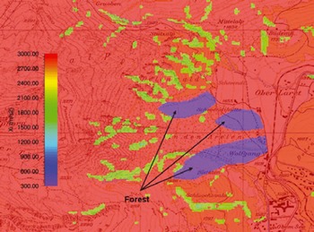
Fig. 7. Spatial variation of friction parameter, ξ. Values generated according to terrain, avalanche volume and return period and vegetation. We assumed a large, 300 year avalanche running on vegetated, open-slope terrain. Forested areas are shown in purple.
We simulated the In den Arelen avalanche with three friction combinations: (1) automatically generated variable μ(x, y) and ξ(x, y) coefficients according to the local terrain, avalanche return period and vegetation; (2) constant μ = 0.22 and ξ = 1500 ms – 2, representing avalanches with a 100 year return period; and (3) constant μ = 0.16 and ξ = 2000 ms−2, representing avalanches with a 300 year return period. The automated procedure found values between 0.16 ≤ μ ≤ 0.27 and 400 ≤ ξ ≤ 3000ms−2. The low ξ values represent forested terrain.
The run-out distance of the In den Arelen avalanche could not be simulated with the 100year return period friction coefficients (Fig. 8). Both the automated procedure and the constant 300 year return period coefficients modelled the run-out distance reasonably well. However, the constant coefficient combination allowed for more lateral spreading (Fig. 8). Because the tangent of the slope angle of the run-out zone is 0.14–0.20, extreme μ = 0.1 6 values were required to reach the observed run-out distance. In both cases, the avalanche depositions were not spread over the entire avalanche track, but were located near the avalanche front. Significant deposition at the tail of the avalanche did not occur. The calculated avalanche depositions at the front, 1–2 m, are in good agreement with the field observations (see section 4.4).

Fig. 8. Three simulation runs with different friction parameters. (a) Maximum flow height and (d) deposition of reference simulation with variable n (0.16–0.27) and ξ (400–3000 ms−2). (b) Maximum flow height and (e) deposition with constant μ = 0.22 and ξ = 1500 ms−2. (c) Maximum flow height and (f) deposition with constant μ = 0.16 and ξ = 2000 ms−2.
Lateral spreading of the central flow arm was restricted by the low ξ values (400 ms−2) of the forested terrain. This led to a realistic simulation of the central arm flow width. However, the forested region in the primary flow direction could not be simulated with this low ξ value. In this case, the breaking effect of the forest was overestimated, causing the avalanche to stop before the observed run-out distance (Fig. 9). Following the Swiss guideline recommendations, we removed the forest cover in the main flowpath.
Fig. 9. Three simulation runs with different forest cover: (a) deposition heights of reference simulation with adjusted forest cover; (b) deposition heights of simulation with complete forest cover; and (c) deposition heights of simulation without forest cover.
4.3. DEM resolution
DEMs can be generated directly from field measurements (e.g. using terrestrial or aerial laser scanning) or obtained directly from a national geo-information centre (e.g. Swisstopo in Switzerland). We performed simulations with an accurate 2.5 m aerial laser-scanning DEM and a 25 m DEM supplied by Swisstopo. In both cases we used a 5 m calculation grid. That is, in one case the calculation grid was coarser than the DEM while in the other it was finer than the DEM. Significant differences were found in respect to snow distribution and run-out distance, mainly for the northern flow arm (Fig. 10). The predicted reach of the central flow arm was obtained (more or less) in both simulations. The northern flow arm clearly travelled further in the 25 m DEM simulation. The northern avalanche arm must pass through undulating, rough terrain, which requires a finer DEM resolution. The path of the centre arm is relatively homogeneous, lessening the importance of the DEM resolution.
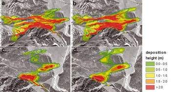
Fig. 10. Two simulation runs with different DEM resolutions. (a) Maximum flow height and (c) deposition (bottom) of reference simulation with a 2.5 m DEM and a calculation grid of 5 m. (b) Maximum flow height and (d) deposition (bottom) of simulation with a 25 m DEM and a calculation grid of 5 m.
4.4. Flow heights, velocities and pressure forces
Little information was available regarding deposition heights in the run-out zone. A hand-drawn sketch from O. Buser provided information about measured deposition heights at the central flow arm (Fig. 11). The measured values correspond well with the calculated deposition heights. A detailed comparison was not conducted, because of the lack of exact positional information. No information about flow velocities or pressure forces was found. However, a pressure range of 30–45 kPa was estimated from the destroyed farmhouse in Figure 1. Calculated pressure forces of 35–50 kPa in the region of the destroyed farmhouse and up to 80 kPa in the forested area west of the farmhouse show good agreement with the estimation (Fig. 11b).
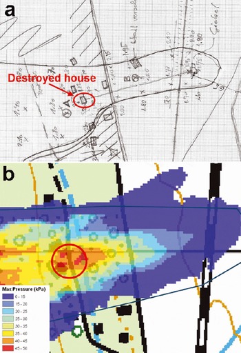
Fig. 11. (a) Hand-drawn sketch of deposition heights in the central flow arm of the In den Arelen avalanche. The red circle indicates the location of the destroyed farmhouse. (b) Pressure forces calculated by RAMMS near the destroyed farmhouse.
5. Discussion and Conclusions
The In den Arelen avalanche event was used to test the two-dimensional avalanche dynamics program RAMMS. The event is typical of many applications, where only sparse data of uncertain quality are available. We applied several novel features of the RAMMS model:
Automated generation and manual modification of potential release areas to model the documented release conditions, which were a function of the meteorological conditions (wind and new snow) on 27 January 1968. We changed the location of the release zones as well as the order in which they released, but did not see any significant effect on the simulation results. This conclusion cannot be generalized to other tracks. It suggests the volume of the event was so large that differences in release scenarios were simply not relevant. We applied the Swiss guideline recommendations for friction coefficients with little modification. We were able to simulate not only the run-out distances but also the general flow direction of all three avalanche arms, as well as impact pressure forces at the destroyed farmhouse. Recently, experimental evidence has been found in Vallée de la Sionne to support the use of these parameters to describe the head, and therefore the extent, of flowing avalanches (Reference Bartelt and BuserBartelt and Buser, 2010).
Aerial photographs were used to define forested regions prior to the avalanche event. We assumed a friction coefficient ξ = 400 m s−2 for forested regions. We could not simulate the run-out of the central avalanche arm with this value. We thus assume that the avalanche destroyed the forest with little frictional expense (Reference Bartelt and StöckliBartelt and Stockli, 2001). In practice, it is recommended to ignore the breaking effect of forests in the main flow direction for extreme avalanches reaching pressure forces >50kPa. Pressure forces of up to 80 kPa in the forested area were obtained in this case study. The In den Arelen avalanche event indicates that this recommendation should be followed.
We specified erosion of the incumbent snow cover, which we assumed to have height hs = 30 cm and density ρs = 200 kgm – 3. With this value we reproduced the deposition heights and extent in the run-out zone which had been recorded by SLF staff immediately after the event. How entrainment should be included in avalanche dynamics calculations remains an open question. With realistic fracture depths, we could not simulate the runout distance without erosion. Of course, the fracture depths could be increased and the run-out distance subsequently correctly modelled.
A fundamental problem that we could not resolve with the In den Arelen case study is the question of DEM and calculation domain resolution. We used both 2.5 and 25 m DEMs and found differences in the deposition distribution but only little discrepancy in the predicted run-out distance of the central arm with a calculation resolution of 5 m. However, the northern arm travelled further with the 25 m DEM, indicating a strong influence of the DEM resolution on the result. Typical calculation resolution varied between 5 and 10 m. We believe that higher-resolution DEMs are required for channelled and inhomogeneous terrain, especially for small avalanche events (volumes <25 000 m3). Large, extreme events, travelling at high speed, appear not to react to small-scale terrain features, suggesting that some simulations can be performed on low-resolution DEMs and yield realistic results. High-resolution DEMs, which are being increasingly obtained from terrestrial or airborne remote-sensing data (Reference Bühler, Hüni, Christen, Meister and KellenbergerBühler and others, 2009), seem to be crucial for small and frequent avalanches. In the same way, wet snow avalanches, travelling at a lower speed than dry snow avalanches, may require a better DEM resolution than dry snow avalanches.
Our In den Arelen case study has shown that RAMMS is a powerful tool for predicting avalanche run-out and complicated flowpaths (avalanche arms) in complex three-dimensional terrain. Additionally, we obtained good estimates for deposition heights and impact pressure forces. The tool contains algorithms for release definition, erosion and friction coefficient selection that can be manually adjusted to allow avalanche experts to test realistic avalanche scenarios. Easy-to-use input and output features allow comparison of historical data with simulation results. Knowledge about possible avalanche arms, lateral spreading and hazard extent are valuable information for practical applications. Further testing of RAMMS, using Vallée de la Sionne measurements and well-documented avalanche events, will help identify model limitations and to improve model performance.


