


1. Introduction
In an earlier study by Reference Morgan, Budd and llusseinyMlorgan and Budd (1978), an attempt was made to estimate the melt rates of Antarctic icebergs from their size distributions , their spatial concentrations in the Southern Ocean, and their movement rates. At that time significant independent data on size distributions were not available for icebergs far from the coast of Antarctica. Thus, it was difficult to take account of the role of factors such as breakage and rollover in the rate of iceberg deterioration. Direct information on iceberg movement rates was also largely confined to areas near the coast rather than the more northerly areas. Also, because of changes in spatial distributions over time, it is important to be able to relate other present-day measurements to iceberg distributions which prevail at present rather than over a long time-scale.
The aim of the present study was to determine the distribution of both concentration and size of icebergs at different stages along drift routes in order to examine processes of deterioration and decay. Furthermore, statistics for regular tabular icebergs were compared with those for irregular ones in order to evaluate the separate effects of melting, breakage, and rollover.
Studies of water temperature were made in order to interpret the derived melt and deterioration rates of the icebergs. The movement of several icebergs in the study region were monitored to provide estimates of average movement rates and drift tracks.
The resul ts are important for a basic understanding of the behaviour of icebergs under present-day conditions and also for the interpretation of conditions which may have prevailed in the past.
2. Region of Study
The iceberg distribution data of Reference NazarovNazarov (1962) and Reference Shil’nikov and Tolstikov YeShil’nikov (1969) indicate that there are some regions where icebergs turn from the coastal east wind drift northwards to the west to east flow of the circumpolar current. These include the Iveddell Sea with the obstruction of the Antarctic Peninsula, the Ross Sea, and in the vicinity of the Kerguelen-Gaussberg ridge near 90°E. This region is discussed here. The iceberg tracks obtained by Reference TcherniaTchernia (1974) as well as recent results from bergs with additional transponders and from large bergs observed by the U.S. Fleet Weather Facility, have clearly defined the iceberg-drift tracks in this region. The main features include a dense concentration near the coast moving westward in the east wind drift and diffusing slowly to the north. Icebergs north of about 64°S. near 90°E. are often caught in eddies taking them first northwards and then to the east near 60°S. in the circumpolar current. Large eddies north of the Amery Ice Shelf also appear to carry icebergs north-east through gaps in the Kerguelen-Gaussberg ridge. Thus the region near the Antarctic coast between 70°E. and 90°E. is the source of most of the icebergs drifting east to the south of Australia.
Typical ship routes are shown in Figure 1, together with the position and year of the most northerly sightings of icebergs from ANARE ship records over the 25-year period from 1954-79. The locations are dependent on the shipping routes, but in general these extremes are south of the contemporary limit line of Reference Shil’nikov and Tolstikov YeShil’nikov (1969). North of latitude 60°S. the concentration of icebergs decreases rapidly and few reach north of 55°S. This is brought out by the concentration/latitude graph obtained from data of the ANARE records in comparison with that of Reference Shil’nikov and Tolstikov YeShil’nikov (1969) for several different longitudes (Fig.2). The lower concentrations shown by the ANARE results along the routes further east indicate deterioration and disappearance of the icebergs as they drift around in the circumpolar current from their source near 90°E.

Fig. 1. Region of study showing typical ANARE voyage routes and most northerly sightings of icebergs with numbers indicating year. Historical (full line) and contemporary (broken line) extents from Shil’nikov’s (1969) compilation are also shown.
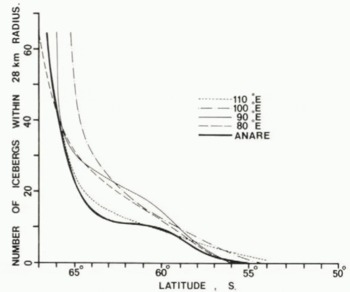
Fig.2. Iceberg concentrations from recent ANARE voyages are shown in comparison with those at different longitudes from Reference Shil’nikov and Tolstikov YeShil’nikov (1969).
For the present study, detailed measurements were made along a route between 120°E. and 60°E., north of 60°S., to compare the distribution and size of icebergs in this region with those in zones further south, especially south of 64°S. in the east wind drift. Thus the history of these icebergs is followed from their east-west coastal flow to their deterioration in the circumpolar flow.
3. Measurements
Since 1977, the data relating to icebergs collected on ANARE voyages include: the number concentration within a 28 km radius (from radar), the widths and visible heights (using a sextant and radar), photographs to determine shapes, ocean temperature measurements, and ship’s location.
The photographs were used to scale accurate heights and widths of the bergs. Typical results of these observations are shown in Figures 3 and 4. No bergs smaller than 50 m in length were included.
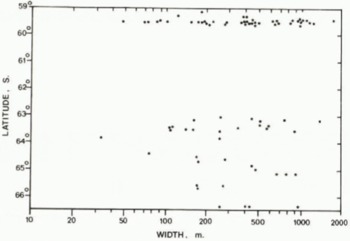
Fig.3. Sample results of iceberg widths as a function of latitude measured on 1977-78 ANARE voyage by .Jacka. Tabular icebergs are indicated by stars.

Fig.4. Observed distribution of iceberg heights for the same samples as in Fig.3. Tabular icebergs are shown by stars.
In February 1979 more detailed measurements were made of three icebergs on which transponders were placed at locations shown in Figure 5. In addition to the observations mentioned above, air photographs were obtained, which provide information on iceberg shape as well as size. The dimensions of the three icebergs were as follows:

Fig.5. Generalized tracks for the three icebergs which were transpondered by ANARE for P. Tchernia. The tracks shown are from 27 February 1979 to 25 January 1980.
Table I Transpondered Icebergs

From that time the locations of these icebergs have been monitored through the satellite transponder system.
4. Iceberg Movement
The movement of the three transpondered icebergs was recorded monthly and is summarized in Figure 5. The general movement of these icebergs is similar to the motion recorded in the same region previously by Reference TcherniaTchernia (1974). These more recent drift tracks, however, have continued farther east, generally just south of 60°S. They, appear to be influenced by the sea-bed topography, with the passage through the same gap in the Kerguelcn-Gaussherg ridge, then following the ridge north before turning east, and following somewhat similar routes as defined by the general bathymetry contours.
Over the same period a large iceberg (about 10 km by 30 km) was plotted by the US Fleet Weather Facility on their Antarctic ice charts from January 1979. Although there was a gap in this record from June to August 1979, it is likely that their iceberg no.4 was the same as D4 which was observed in September and then monitored up to January 1980. The track is similar to that of the three smaller icebergs described above except that the large iceberg followed the Kerguelen-Gaussberg ridge further north and west before turning east, reaching 55°S., 84°E.
Further information relevant to iceberg drift patterns has been supplied during 1979 from the drifting buoys of the First GARP Global Experiment (FGGE). The buoys located near the iceberg tracks show similar movements, and also appeared to be influenced by the sea-bed topography.
5. Iceberg Deterioration
The observations and photographs of the icebergs provide some insight into the different mechanisms for iceberg deterioration besides simple melting. These include wave erosion of the firn and caving, calving of edges to form shoulders, splitting or breaking, tilting, and rollover.
Although the act of rollover is not often observed, ample evidence for its existence is obtained from icebergs displaying sides or bases as upper surfaces, usually in an advanced stage of deterioration. The presence of hasal morainic material and handed layered ice may indicate that rollover or at least turning on to one side has occurred.
Examples of these forms of deterioration are shown in Figure 6 which also illustrates the difficulty in determining clear measurements of height or width for irregular icebergs. With this in mind the statistical distribution studies here have distinguished between the regular tabular and the irregular icebergs.

Fig.6. Photographs showing stages of iceberg deterioration. Supplied from the official ANARE collection held by the Antarctic Division.
6. Size Distributions
Statistical frequency distributions and cumulative distributions have been obtained from the data of the type shown in Figures 3 and 4. Figures 7 and 8 show, respectively, the relative cumulative distributions of the iceberg widths and heights for latitudes S9.5°S. and 64°S. compared to the results given by Reference RomanovRomanov (1973) for north and south of 65°S. off east Antarctica. The results of ANARE measurements of height distribution in the region of 64°S. are similar to those of Romanov except that fewer of the extreme heights were obtained with tabular icebergs. The distribution at 59.5°S. shows a definite decrease in height of about 10 m, but as discussed later all of this decrease cannot be attributed to melting.

Fig.7. Cumulative relative frequency distribution of iceberg heights (all icebergs) observed on ANARE voyages for latitudes 64 and 59.5°S. compared to distributions given by Reference RomanovRomanov (1973).
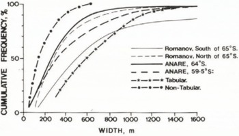
Fig.8. Cumulative relative distribution of iceberg widths for latitudes 64 and 59.5°S. (all icebergs) obtained on ANARE voyages compared to those of Reference RomanovRomanov (1973) . Differentiation of ANARE distribution into tabular and non-tabular icebergs is also shown.
The distribution of widths at 64°S. and 59.5°S. are more similar to the Romanov distribution N. of 65°S. than to that S. of 65°S., as would be expected from the rapid change of concentrations north of 65°S. The ANARE distributions also show an increase in mean size towards the north which is due to a decrease in numbers of icebergs above the 50 m size limit. This is further supported by considering the separate relative distributions for the tabular and the non-tabular or irregular icebergs at 59.5°S. Here the tabular bergs have an even greater median width than the Romanov distribution south of 64°S. although few of the very large icebergs were observed by ANARE. The irregular icebergs, on the other hand, have a mean length of only about 150 m, representing, on the whole, advanced stages of decay.
The relative frequencies should be combined with the actual number concentrations per unit area, as shown in Figure 2, in order to record real changes in iceberg sizes along the drift tracks. Furthermore, when comparing concentrations at different latitudes, the divergence of the meridians towards the north, which also reduces the number per unit area, should be considered. Iceberg size concentrations per unit area (28 km radius circle), adjusted for divergence to lat. 64°S., are shown for heights and widths in Figures 9 and 10.

Fig.9. Iceberg frequency concentration of heights (per 20 m interval) adjusted for divergence to 64°S. as observed from ANARE voyages for 64 and 59.5°S.
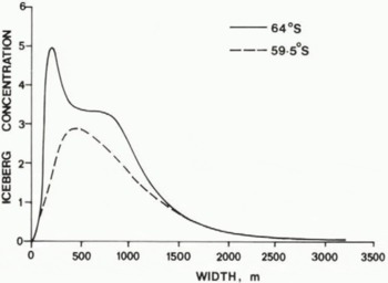
Fig.10. Corresponding distribution of iceberg widths from the sample of Figure 9, expressed as a concentration per width intervals increasing by a factor of two, viz., 50-100, …, 1600-3200 m.
The frequencies of widths of large tabular icebergs for the different latitudes are very similar but there is a marked decrease in frequency as the sizes of the icebergs decrease down to the size limit at 50 m. This decrease cannot be due to melting alone.
There is a small but significant decrease in the frequency of the largest heights, a large decrease in numbers near the mean height, and an increase in the smaller heights. Although the shifts at the end of the spectrum are compatible with a general reduction of 5 m from melting, the decrease around the mean height is too large for that and so will also be considered in regard to the consequences of splitting and breakage.
7. Iceberg Breakage Rates
Although the data on size distributions of icebergs presented here indicate possible breakage activity, more data using larger samples would be required to determine the changes precisely. Hence only the simplest considerations are presented. in the case of icebergs of large horizontal dimension compared to their thickness, the melt or wastage at the edges makes little difference initially to the change in dimensions, and so their survival is limited by their decrease in thickness until they become so thin that they break up. The side wastage does not become a problem until the horizontal dimensions arc about twice the thickness. Thus the basal melt rates and breakage rates are very important for the deterioration of large bergs.
If there were no melting, and large bergs deteriorated by breakage alone, then a frequency distribution doubling for each halving of size could be expected. Even larger numbers of smaller bergs could be expected if they entered from the source. The measured width frequencies Shom in Figure 10 suggest that this may be true down to about 800 m, but, at widths less than that, melting must account for an increasing proportion of the deterioration.
Suppose then a size distribution is expressed as a function of widths decreasing by a factor of two. Let it be assumed that breakage results in two similarly sized pieces. Then the breakage of a certain number of icebergs from one interval contributes double that number to the interval below. This can be expressed quantitatively as follows: Let B(x) be the breaking rate (i.e. the proportion of icebergs breaking in two per unit time) in the log interval centred on x, where x is a measure of the horizontal dimension of the iceberg. Let f 1(x) be the initial number of icebergs in that interval and f 2(x) the number after unit time.
Then
By choosing x = X sufficiently large so that f1 (2X)is negligible,
and
Thus B(X) can be found from Equation 2 and the breaking rate at subsequent half intervals from Equation 3. This technique has been used to estimate the average breaking rates as a function of size from the width distributions given in Figure 10.
Table II shows the mean breaking rates over the representative time between the two distributions. From the observed tracks of the transpondered icebergs this mean time is estimated as 0.8 a with a spread of ≈ ±0.3 a over the region of the observed iceberg distribution near the lat. 59.5°S. route. This allows a conversion to typical half-lives for the icebergs in each interval. The results suggest an increasing half-life with iceberg size ranging from ≈ 0.5 a for bergs about 200 m wide to ≈ 4 a for bergs 1.6 km wide. This apparent dependence on width may be spurious because the widths in these samples are correlated with the heights and therefore the increase with width may be associated with increasing thickness. The mean heights and estimated thicknesses arc therefore also shown.
Table II Iceberg Breakage Rates

Low melt rates will reduce the thickness of very large icebergs, eventually allowing higher breakage rates. Thus many large icebergs spend a number of years moving around the Antarctic coast, but after reaching the warmer waters break up rapidly.
For icebergs greater than 800 m width, breakage would seldom result in a rollover, but this is likely for smaller icebergs. It is most likely for those icebergs where the half width is smaller than the thickness. The height distributions shown in Figure 9 indicate that this process does take place. There is little change in the large heights but a large decrease in the median heights along with an increase in heights of about half that size. This is compatible with splitting of icebergs of comparable width to thickness ratios, followed by a rollover on to their sides, with a resulting increase in numbers of bergs of half the thickness. Thus, in Figure 9 when icebergs about 400-600 m wide and 60 m high break up, icebergs of about half that height could result. Further breakage, rollover, and melting can follow the initial breakage and cause a more rapid deterioration, resulting in the observed decrease in concentration of those sizes and a shift of the sizes to below the 50 m size limit.
This analysis so far neglects the length to breadth ratios of the icebergs, and the influence of the melt from the sides on this ratio. As the icebergs become smaller from side melt at equal rates m in both directions, the length l to breadth b ratio increases as
provided rollover does not occur. This means that breakage which can be expected to be perpendicular to the longest dimension can more readily occur as the length to breadth ratio increases while at the same time the thickness decreases. Thus, breakage tends to counteract the production by melting of more elongated shapes which could then explain the tendency noticed by Dmitrash (1973) for mean iceberg length to breadth ratios of between 1.5 and 1.6. A ratio of about 1.4 would allow a continual halving perpendicular to the long axis without changing the ratio. Thus breakage can be expected to tend to maintain such an aspect ratio, in conjunction with melting, until rollover occurs.
8. Iceberg Rollover
Once the smallest horizontal dimension Y of a tabular iceberg becomes comparable to the vertical dimension Z then the iceberg is likely to roll over as additional side wastage occurs. If the melt rates m of the base and sides are comparable then the time to reach rollover from melting alone is given by
or
.
Rollover is not reached if ![]() or if Y
0 > 2 Z
0.
or if Y
0 > 2 Z
0.
Once rollover has occurred the decrease in the horizontal dimension can lead to further rollovers. The thinning of the iceberg is increased on the average by twice the rate for half the time, which amounts to an effective 50% increase in vertical melt rate. This however is still less than a continued double rate in the third (longest) dimension which tends to lead to more cubic shapes, but with possible pinnacles occurring from upright corners.
The condition that Y < 2 Z also allows rollover to occur as a result of breakage. Thereafter any additional breakage would also lead to rollover. Thus the melting, breakage, and rollover tend to work together in the ultimate rapid decay of icebergs. The numerical data for melt rates and breakage rates combined with rollover can provide the basis for a simple model of iceberg deterioration’which should then lead to the observed size distributions and decay rates given here.
9. Historical Data
It is interesting to place the present-day iceberg distribution over the Southern Ocean in perspective with that observed in the past. Reference HerdmanHerdman (1959) has summarized some of the earliest recorded observations of Antarctic icebergs, which were made by Captain James Cook from 1772 onwards. The locations of Cook’s sightings of icebergs are compatible with the contemporary compilation of iceberg concentrations described by Reference Shil’nikov and Tolstikov YeShil’nikov (1969). Reference TowsonTowson (1859) reported a considerable increase in number of icebergs in the Southern Ocean for several months in 1854-55. Iceberg sightings of that short period were included in the summary by Reference NazarovNazarov (1962). These accounts suggest a considerably greater number of icebergs in earlier times compared to the present. Russell (Reference Russell1895, Reference Russell1897) reported a second period in 1888-97 of increase of iceberg numbers In the Southern Ocean. A map based on Russell’s map for the period 1888-97 is shown in Figure 11. The icebergs in some locations are some 10° of latitude further north than the most northerly sightings in recent times. Reference NazarovNazarov (1962) did not include Russell’s data in his map.
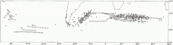
Fig.11. Sightings of icebergs during 1888 to 1897 reported by Reference RussellRussell (1895, Reference Russell1897). Numbers indicate last digit of year of sighting. Also shown is the drift track (D) of the abandoned Dumbartonshire from August 1894 to March 1895.
Reference MaksimovMaksimov (1961) included a comparison of Russell’s data with contemporary iceberg sightings to indicate the large changes between them. Reference Shil’nikov and Tolstikov YeShil’nikov (1969) included the data from Nazarov’s compilation as well as that of Maksimov in his analysis and also distinguished past data from contemporary observations. The earlier observations provide a useful indication of iceberg decay rates in regions further north, with higher sea temperatures, than those where icebergs are found today.
Although Reference Maksimov and LykovaMaksimov and Lykova (1975) suggest that the Antarctic convergence may also move north with the icebergs, that is not considered to be the case here, because the decay rate of the icebergs increases more rapidly as they drift north as one would expect from the higher water temperatures. As an example of the influence of the temperature of the ocean on iceberg distribution, Figure 12 shows Reference NazarovNazarov’s (1962) iceberg distribution superimposed upon a chart of ocean temperatures at 200 m depth from Reference Gordon and GoldbergGordon and Goldberg (1970). The isotherms reflect the current patterns, with the Antarctic convergence near the 5°C isotherm. The iceberg distribution also follows the current flow, but there still appears to be some diffusion to the north. These data have been used here together with the results from the FGGL drifting buoys to estimate melt rates.

Fig.12. Distribution of iceberg sightings reported by Reference NazarovNazarov (1962) superimposed upon contours of mean ocean temperatures (°C) at 200 m depth as given by Reference Gordon and GoldbergGordon and Goldberg (1970).
10. Melt Rates
A scheme for calculating melt rates of icebergs from their spatial distribution, initial size distribution, and drift velocities was described by Reference Morgan, Budd and llusseinyMorgan and Budd (1978). The aim here is to reassess these results in the light of considerations of breakage, rollover, and more recent data on iceberg and buoy velocities and tracks.
Briefly, the calculation of the melt rates can be considered as the inverse to that of deriving the iceberg size and spatial distributions from the melt rates. That is to say, suppose the melt rates (of base or sides) is given, as a function of temperature, along with an initial size distribution, and the paths and speeds of the iceberg drift. It is assumed that the paths can be superimposed onto an appropriate ocean temperature chart so that the melt rate and total melt occurring along the path can be calculated. From the initial size distributions, the size and number of the icebergs along the route can be calculated from the accumulated melting if other factors are ignored.
The inverse problem is to calculate the melt rates for each element of path length over a temperature interval from the change in the number concentration (e.g. as given by Shil’nikov) and the initial iceberg size distributions.
During drift, the size distribution (actual numbers per unit size interval) changes by a shift along the size axis (thickness or width) depending on the melt rate. This results in a decrease in total number concentration by a loss of icebergs from the smaller sizes. Both of these features (i.e. the change in total number as well as number per unit size interval) effect the change in the percentage frequency size distribution along the route. Starting from the source the change in total numbers for each element of path length was calculated on the assumption that the size distribution changed by the shift described above. From this shift (from the total melt) and the travel time the melt rates are calculated. The most important unknown factors in this calculation are the rates of iceberg drift and the contribution of other processes such as breakage and rollover to the decreasing numbers of bergs.
The results of Reference Morgan, Budd and llusseinyMorgan and Budd (1978) were reassessed using the FGGE drifting buoy data as indicators of possible drift speeds. This resulted in the upper limit full curve of Figure 15. However, icebergs extend to much greater depths than buoys and can be expected to drift more slowly due to the change of currents with depth. The upper curve in Figure 15 is therefore considered as an upper limit to the melt rates. The lower curve results from taking breakage and rollover into account, which gives a rate of deterioration greater than would occur from melting alone, and therefore implies lower melting rates.

Fig. 13. Variation of iceberg concentration (per 2°C interval) with ocean temperature at 200 m depth as derived from data of Figure 12 and Reference Shil’nikov and Tolstikov YeShil’nikov’s (1969) compilation.

Fig.14. Observed temperature depth profiles from XBT measurements along 1977-78 ANARE voyage between Melbourne and Mawson on which Jacka’s data were obtained. (Courtesy of Dr J.S. Boyd, Antarctic Division.)

Fig.15. Bounds of iceberg melt rates obtained from the present analysis in comparison with those obtained in the earlier study by Reference Morgan, Budd and llusseinyMorgan and Budd (1978), which gave melt rates for the base (•) and the sides (*).
For the more northerly regions, where Shil’nikov’s concentrations approach zero, the change in numbers along the drift tracks from Nazarov’s and Russell’s data has been used. Although these iceberg sightings are to some extent dependent on the shipping routes, the more northerly regions were within the well-travelled shipping lanes and are therefore assumed to provide a reasonable representation of the limits of iceberg drift. For these sightings, the initial size distribution was taken from Nazarov’s observations in the Weddcll Sea which appears to be the major source of these icebergs, although a few appear to have come through Drake Passage.
Using the iceberg distributions of Reference NazarovNazarov (1962) and Russell (Reference Russell1895–Reference Russell97) together with the 200 m depth temperature data and the FGGE drifting buoy movement rates, the melt rate of the icebergs in the various temperature zones (Fig. 12) has been estimated. As an indication of the rapid decrease of the iceberg concentration with temperature, Figure 13 shows the results obtained from Figure 12 using the Nazarov distribution as a function of the 200 m depth temperature.
Taking account of breakage and rollover as well as melt only alters the results slightly. For the large icebergs basal melting is still the primary factor in their deterioration, Eventually breakage occurs, followed by rollover and more rapid deterioration. The increase in the decay rate however is only about 50% and occurs only in the final stages. This seems to account partly for the rather sharp cut-off at the limits of the iceberg spatial distribution.
The calculated melt rates for 60°S., where the measured iceberg concentrations and size distributions as describe above were obtained, agree with those previously obtained By Reference Morgan, Budd and llusseinyMorgan and Budd (1978) for temperatures around 1° to 2°C. The temperatures measured to 450 m depth along the royte from Australia are shown in Figure 14.
Further north there is a wide range of scatter in the estimates of melt rates, but it is possible to put reasonable bounds on these as shown in Figure 15. Here there is a suggestion of somewhat higher melt rates at the higher temperatures than those given by Reference Morgan, Budd and llusseinyMorgan and Budd (1978) but the results are not sufficiently precise to be definite. Nevertheless, it is possible to say that if the melt rates were much higher or lower than these bounds then either the icebergs could not drift so far or would travel much farther than observed.
In order to obtain more accurate results precise measurements on a number of transpondered icebergs would be useful with subsequent re-measurcmcnt at a later date to determine changes in dimensions accurately.
11. Conclusions
Twenty-five years of observation from ANARE ships have established a contemporary limit of iceberg extent south of Australia. The movement of transpondered icebergs and the tracks of drifting buoys have established a source and decay drift path of icebergs moving north and east from near 90°E.
Detailed measurements of size distributions of icebergs with accompanying photographs along this drift route enabled a picture to be obtained of the processes and rates of decay. Definite indications of breakage allow an estimate to be made of breakage rates and half-lives of icebergs of different sizes. The breakage rates appear to increase with decreasing iceberg thickness which then leads to rollover and more rapid deterioration of the original height from melting. The data provide the basis of a numerical model for iceberg decay.
Although spatial distributions of icebergs have been more extensive for limited periods over the past two centuries, the limits of the extent can be explained in terms of the iceberg drift, melt, breakage, and rollover decay processes given here. These iceberg distributions thus provide reasonable bounds of the melt rates versus temperature over that limited temperature range in which the icebergs occur naturally.
Acknowledgements
The authors wish to express their appreciation to all the ANARE cxpeditioners who assisted in the collection of data presented in this paper, in particular, G. Akerman, T. Hamley, D. Sheehy, and J. Wilson.
Thanks are also due to Dr J.S. Boyd of Antarctic Division who made available unpublished data on Southern Ocean temperature-depth profiles, and to J. Birch of the Meteorology Department, Melbourne University, who assisted in the compilation and statistical analysis of the data.


