


1. Introduction
Interdisciplinary explorations of the impact of the Covid-19 pandemic play a key role in decision-making by local and national government policymakers, international organisations, healthcare providers, insurance companies and other agencies. The availability of good prediction models could help to provide critical responses to impact on the public health, social care and economic systems. Several methodologies have been proposed based on different approaches, assumptions, metrics and time horizons of the predictions. These differences mean that it is not straightforward to identify which models produce the best performance (for example, see Peracchi et al., 2020; Harvey et al., 2020; Ferguson et al., Reference Ferguson, Laydon, Nedjati-Gilani, Imai, Ainslie, Baguelin, Bhatia, Boonyasiri, Cucunubá, Cuomo-Dannenburg, Dighe, Dorigatti, Fu, Gaythorpe, Green, Hamlet, Hinsley, Okell, van Elsland, Thompson, Verity, Volz, Wang, Wang, Walker, Walters, Winskill, Whittaker, Donnelly, Riley and Ghani2020; MIT, 2020; Li et al., Reference Li, Bouardi and Lami2020 and Gu, Reference Gu2020). Nevertheless, a common feature of the different methodologies consists in investigating “how will the temporarily stressed mortality rates change the post-Covid-19 mortality rates?” (Andersson et al., 2021).
The mortality stress or shock due to the pandemic has been modelled and explained in various ways. In Milevsky (Reference Milevsky2020), the total mortality rates during the coronavirus period have been described as strictly proportional to normal mortality rates, reflecting a parallel shift of the normal (Gompertzian) term structure. Spiegelhalter (Reference Spiegelhalter2020) similarly investigates the profile of the excess of deaths due to the pandemic shock as a parallel shift in the curve of log mortality rates and as an upward shift in the current age.
As argued by Schnurch et al. (2021), the mortality shocks caused by the Covid-19 pandemic could represent transitory mortality jumps, rather than consisting of long-term changes to the levels of the mortality rates. These authors also assume that Covid-19 leads to a log-parallel shift of death rates which is assumed to be constant, i.e. mortality rates increase by a multiplicative factor which is independent of age. Schnurch et al. (2021) note that, in the context of the Lee Carter mortality model, it will be necessary to assess the violation of the usual normal distribution hypothesis for the first-differenced period effects. Vanella et al. (Reference Vanella, Basellini and Lange2021) propose an approach to estimate the excess mortality due to Covid-19, on the basis of the Lee-Carter model by estimating principal components on multi-population mortality data. Cairns et al. (Reference Cairns, Blake, Kessler and Kessler2020) estimate excess mortality for England and Wales, focussing on the more risky subgroup of the population. They compute a baseline model, that is a Gompertz mortality model, by projecting mortality rates for all-causes of death corrected by a multiplicative adjustment factor for individuals aged over 75. They consider different mortality scenarios for the course of the pandemic and, compare the results with the observed data, and define the role of some risk factors in Covid-19 mortality, such as, age, gender, economic deprivation and respiratory diseases. They also investigate the indirect consequences of the pandemic, in terms of the healthy state of individuals who survive infection.
In the literature, the linkage between longevity and morbidity has been extensively examined, where the random changes in individual frailty occur due to the stochastic processes of physical deterioration (Fong et al., 2015). The individual’s relative susceptibility to death compared to a standard has been described by the traditional frailty models (introduced by Vaupel et al., Reference Vaupel, Manton and Stallard1979), where it is assumed that an individual’s frailty is fixed throughout a person’s lifetime and does not vary with age. A number of studies have extended this model (see for example, Yashin et al., Reference Yashin, Vaupel and Iachine1994; Lin and Liu, Reference Lin and Liu2007 and Su and Sherris, Reference Su and Sherris2012), by assuming that frailty is not fixed, and that the susceptibility to death follows an ageing process recognising the effects of physiological changes and environmental influences. In Banerjee et al. (Reference Banerjee, Pasea, Harris, Gonzalez-Izquierdo, Torralbo, Shallcross, Noursadeghi, Pillay, Sebire, Holmes, Pagel, Wong, Langenberg, Williams, Denaxas and Hemingway2020), Covid-19 multiplies the “normal risk” of dying in the following year, introducing a fixed additional relative risk from Covid-19 to be applied to the 1-year mortality rate based on age, sex, and pre-existing medical conditions. In the discussion about the future risks of getting Covid-19 and dying, Spiegelhalter (Reference Spiegelhalter2020) refers to “some selection of frail elderly people, bringing their deaths forward and leaving a temporarily more resilient cohort”.
In this paper, we focus on the empirical evidence from studies in different countries pointing out that many of those who have died from coronavirus would have died anyway in the relatively near future due to their existing frailties or co-morbidities, the phenomenon being described as an acceleration in timing as in Cairns et al. (Reference Cairns, Blake, Kessler and Kessler2020).
Inspired by the work of Cairns et al. (Reference Cairns, Blake, Kessler and Kessler2020), we assume that the mortality shocks are related to a group of individuals with co-morbidities. According to this hypothesis, the mortality shock presents a specific characterisation, which has a causal connection with pre-existing conditions. The acceleration represents the underlying idea that the deaths are ‘accelerated’ ahead of schedule due to Covid-19. Starting from this suggestion, we forecast the future mortality acceleration in a stochastic setting for the Italian population, on the basis of the relative frailty deterioration due to the presence of the co-morbidities at Covid-19 diagnosis and the future trajectory of infection rates. The idea is that neither Covid-19 infection nor the presence of co-morbidities is its own cause of death, but that the two factors must be considered as contributing causes of mortality. In other words, the pandemic shock does not uniformly affect all the population, but only the part with a greater risk of mortality. Further, we consider the financial impact on some standard life insurance contracts, in order to detect the magnitude of such financial consequences. The effects of the Covid-19 pandemic on the insurance market are quantified by comparing the baseline premium and the adjusted premium, by developing some metrics measuring the extra premium in case of the mortality acceleration.
We focus attention on Italian data because Italy is a particular case for the first Covid-19 wave (in the period between February and May 2020), being the first European country to be severely hit by Covid-19 infection and to introduce hard restrictions to reduce infections. Moreover, in Italy, the first and second waves have been profoundly different in terms of incidence and geographical spread, and some authors have studied the differences in terms of excess mortality and immunity achieved (for instance, see Carletti and Pancrazi, Reference Carletti and Pancrazi2021). Moreover, for the data relating to these two waves, it is possible to highlight the effects of the co-morbidity conditions on mortality due to Covid-19 thanks to the availability of clinical data relating to Italian hospitals and medical centres.
The structure of the paper is as follows. Section 2 is devoted to the background and the motivation of the paper. Section 3 proposes the Accelerated Mortality Model. In Section 4, we present some acceleration metrics for actuarial evaluations. The main empirical findings are presented and discussed in Section 5 and Section 6 provides some concluding comments.
2. Background and Motivation
There is great uncertainty in how future mortality may be impacted by the pandemic and hence various views on this impact have resulted. As shown in a SOA survey (2021), in many cases, the impact of COVID-19 has not yet been studied or there is not yet data available here was no observable impact.
So far, the literature mainly detects the short-term effects of the Covid-19 on mortality projections. According to Kyriakou (Reference Kyriakou2021), it is too soon to understand if the recent 2020 mortality spike will affect the downward trend in projected mortality rates in the longer term. The ISEG 2021 report highlights that “many CMI users believe that the 2020 mortality experience is one of a kind and most likely an unwise guide to future mortality improvements”. The 2020 data could represent a sort of “outlier” that would lead to contort projections (Gaches, Murray & Scott, Reference Gaches, Murray and Scott2021). According to Daneel & Palin (Reference Daneel and Palin2021) including the 2020 data in the analysis could cause more than 10 months decrease in the life expectancy for a 65-year-old female and almost 15 months fall for 65-year-old males when compared to the CMI 2019 model life expectancies.
Recently, there is a growing interest in studying the long-term effect of the Covid-19 on the future evolution of the mortality. Indeed, there is an active discussion around “long COVID” in many fields; above all, the medical research investigates the point. Nevertheless, the actuarial community too considers the possibility that persons who were infected by the virus could experience a negative impact on their health that remains after surviving it (American Academy of Actuaries, 2020), for example, because of decreased lung capacity (Palin, Reference Palin2021), by causing higher mortality rates in the future. Within this line of thinking, “actuaries and trustees could be motivated to consider that mortality improvements may decrease in the future and that the impact of the virus might not just be a short-term impact” (ISEG, 2021). On the other hand, the structural effects of the Covid-19 could depend on the healthier habits adopted to control the spread of the disease and the increased awareness of infection risks which could decrease deaths from the annual flu in the future (Caine, 2020b). In other words, it could involve a positive long-term impact on future mortality evolution. The American Academy of Actuaries (2020) points out that for example, “more careful handwashing and mask-wearing can reduce the spread of other illnesses now and even new ones in the future”.
In other research, we also deepened the long-term effects of the Covid-19 on the individual frailty and its systemic relationship with the mortality (Carannante et al., 2022). Our outcomes, in line with an increasing disabled life mortality (ISEG survey, 2021), underline a long-term effect of the Covid-19 on the future mortality, having been averaged out by the frailty and represent more stable estimates in describing the evolution of the phenomenon.
Some studies show that many of those who die from coronavirus would have died anyway in the relatively near future due to their existing frailties or co-morbidities. The acceleration of the mortality conceives the underlying insight according to deaths are ‘accelerated’ ahead of schedule due to Covid-19 (Cairns et al., Reference Cairns, Blake, Kessler and Kessler2020). From a medical perspective, other studies on COVID-19 have consistently shown that older age and comorbidity are major risk factors for adverse outcomes and mortality (Zhou et al., Reference Zhou, Yu, Du, Fan, Liu, Liu, Xiang, Wang, Song, Gu, Guan, Wei, Li, Wu, Xu, Tu, Zhang, Chen and Cao2020. Some authors argue that comorbidities are associated with a considerably increased risk of mortality (Chen et al., Reference Chen, Mao and Leng2014 and Clegg et al., Reference Clegg, Young, Iliffe, Rikkert and Rockwood2013). Starting from these interesting cues of reflection, we forecast the future mortality acceleration in a stochastic setting for the Italian population, on the basis of the relative frailty deterioration due to the presence of the co-morbidities at Covid-19 diagnosis.
3. Accelerated Mortality Model
In our study, we assume that the mortality shocks due to Covid-19 are specific. Based on empirical evidence from England and Wales, as shown in Cairns et al. (Reference Cairns, Blake, Kessler and Kessler2020), we start from the hypothesis that the mortality shocks lead to an acceleration in the timing of mortality with particular emphasis on the sub-group of a population with co-morbidities. Following Cairns et al. (Reference Cairns, Blake, Kessler and Kessler2020), we consider the proportion $\pi \!\left( {x,t} \right)$
who will die from Covid-19, out of the deaths expected or ‘scheduled’ to die at time t which is defined as the baseline cohort-based curve of deaths
$\pi \!\left( {x,t} \right)$
who will die from Covid-19, out of the deaths expected or ‘scheduled’ to die at time t which is defined as the baseline cohort-based curve of deaths ${\rm{\;}}d\!\left( {x,t} \right)$
. This can be expressed in a deterministic setting by the following formula:
${\rm{\;}}d\!\left( {x,t} \right)$
. This can be expressed in a deterministic setting by the following formula:
 \begin{align} \pi \!\left( {x,t} \right) = \frac{{\alpha \!\left( x \right)}}{{\rho \!\left( {x,t} \right)}}exp\!\left( {\frac{{ - t}}{{12\rho \!\left( {x,t} \right)}}} \right)\end{align}
which, in Cairns et al. (Reference Cairns, Blake, Kessler and Kessler2020), relies on “the idea that people who are expected to die sooner rather than later are more likely also to die from Covid-19 if they have contracted the virus”. The formula represents the concept of acceleration. Here, the amplitude parameter $\alpha \!\left( x \right)$
represents the proportion of Covid-19 deaths at age x and the reach parameter
$\alpha \!\left( x \right)$
represents the proportion of Covid-19 deaths at age x and the reach parameter $\rho \!\left( {x,t} \right)$
represents the loss in terms of life expectancy at age x due to Covid-19 deaths.
$\rho \!\left( {x,t} \right)$
represents the loss in terms of life expectancy at age x due to Covid-19 deaths.
It is noteworthy that the shape of $\pi \!\left( {x,t} \right)$
is “chosen to reflect the observation that most people who die from Covid-19 have existing significant co-morbidities” (Cairns et al., Reference Cairns, Blake, Kessler and Kessler2020).
$\pi \!\left( {x,t} \right)$
is “chosen to reflect the observation that most people who die from Covid-19 have existing significant co-morbidities” (Cairns et al., Reference Cairns, Blake, Kessler and Kessler2020).
Our perspective is to model and interpret the effect of Covid-19 on mortality during the current emergency and post-pandemic. Hence, the acceleration requires modelling of the dynamics of the infection rate and the link between Covid-19 and frailty by age which, in particular, affects people with co-morbidities that significantly present an extra risk of death relative to healthy individuals of the same age (i.e., with no significant co-morbidities). Accordingly, we propose a new measure of the acceleration where the correction of the stochastic projection of mortality depends on the frailty and the infection rate for each age cohort. In order to express the acceleration for specific age $x$
at time
$x$
at time $t,{\rm{\;\;}}A\!\left( {x,t} \right),{\rm{\;}}$
in a stochastic setting, we model:
$t,{\rm{\;\;}}A\!\left( {x,t} \right),{\rm{\;}}$
in a stochastic setting, we model:
 \begin{align}A\!\left( {x,t} \right) = q\!\left( {x,t} \right)*{\pi ^S}\!\left( {x,t} \right)\end{align}
Formula (2) is defined by the product of three factors: $q\!\left( {x,t} \right)$
and
$q\!\left( {x,t} \right)$
and ${\pi ^S}\!\left( {x,t} \right)$
that is equal to
${\pi ^S}\!\left( {x,t} \right)$
that is equal to $\lambda \!\left( {x,t} \right)*SIRf\!\left( {x,t} \right)$
.
$\lambda \!\left( {x,t} \right)*SIRf\!\left( {x,t} \right)$
.
The infection rate $\lambda \!\left( {x,t} \right)$
and the smoothed implied infection rate
$\lambda \!\left( {x,t} \right)$
and the smoothed implied infection rate $SIRf\!\left( {x,t} \right)$
are both random variables.
$SIRf\!\left( {x,t} \right)$
are both random variables. $\lambda \!\left( {x,t} \right)$
is a random variable since it is estimated using the Gompertz dynamic model, that is a stochastic model with time-varying parameters.
$\lambda \!\left( {x,t} \right)$
is a random variable since it is estimated using the Gompertz dynamic model, that is a stochastic model with time-varying parameters. $SIRf\!\left( {x,t} \right)$
is a random variables, since it is estimated by combining three variables: a measure of accelerated deaths
$SIRf\!\left( {x,t} \right)$
is a random variables, since it is estimated by combining three variables: a measure of accelerated deaths $A\!\left( {x,t} \right)$
, obtained by observed data on deaths due to Covid-19 in 2020, thus a non-random variable, a measure of mortality for all causes
$A\!\left( {x,t} \right)$
, obtained by observed data on deaths due to Covid-19 in 2020, thus a non-random variable, a measure of mortality for all causes $q\!\left( {x,t} \right)$
, estimated using a Renshaw-Haberman model (Renshaw and Haberman, Reference Renshaw and Haberman2003), thus a random variable, and the infection rate
$q\!\left( {x,t} \right)$
, estimated using a Renshaw-Haberman model (Renshaw and Haberman, Reference Renshaw and Haberman2003), thus a random variable, and the infection rate $\lambda \!\left( {x,t} \right)$
, described above and a random variable.
$\lambda \!\left( {x,t} \right)$
, described above and a random variable. $q\!\left( {x,t} \right)$
and
$q\!\left( {x,t} \right)$
and $\lambda \!\left( {x,t} \right)$
are not simulated but the out-of-sample forecasts of the relative models.
$\lambda \!\left( {x,t} \right)$
are not simulated but the out-of-sample forecasts of the relative models.
Gompertz dynamic model is defined in Appendix; Smooth Implied Relative Frailty, or $SIRf\!\left( {x,t} \right)$
, which represents the comorbidity at Covid-19 diagnosis condition for the age
$SIRf\!\left( {x,t} \right)$
, which represents the comorbidity at Covid-19 diagnosis condition for the age $x$
at time
$x$
at time $t$
.
$t$
. $SIRf\!\left( {x,t} \right)$
is calculated using the observed data. Considering formula (2), the implied frailty is the value estimated backwards by using the historical values of Covid-19 mortality rates as a measure of acceleration
$SIRf\!\left( {x,t} \right)$
is calculated using the observed data. Considering formula (2), the implied frailty is the value estimated backwards by using the historical values of Covid-19 mortality rates as a measure of acceleration $A\!\left( {x,t} \right)$
, along with the all-cause mortality rate
$A\!\left( {x,t} \right)$
, along with the all-cause mortality rate $q\!\left( {x,t} \right)$
and the infection rate
$q\!\left( {x,t} \right)$
and the infection rate $\lambda \!\left( {x,t} \right)$
. The implied frailty is then used as a forward-looking measure, and, in addition, we have used a p-spline smoothing model to obtain smoothed estimates of the implied frailty as a function of age.
$\lambda \!\left( {x,t} \right)$
. The implied frailty is then used as a forward-looking measure, and, in addition, we have used a p-spline smoothing model to obtain smoothed estimates of the implied frailty as a function of age.
1. Acceleration Metrics in Insurance. The mortality shocks due to the pandemic will have a financial impact on the life insurance industry, depending on the specific contracts being considered. We define the Mortality Acceleration ${}^{MA}{}_{\!\!t}{\vartheta _x}$
as the spread between the mortality projections:
${}^{MA}{}_{\!\!t}{\vartheta _x}$
as the spread between the mortality projections:
 \begin{align}{}^{MA}{}_{\!\!t}{\vartheta _x} = Ac{c_{q\!\left( {x,t} \right)}} - Bas{e_{q\!\left( {x,t} \right)}}\end{align}
the $Ac{c_{q\!\left( {x,t} \right)}}$
being the accelerated future mortality estimate for an individual aged
$Ac{c_{q\!\left( {x,t} \right)}}$
being the accelerated future mortality estimate for an individual aged $x$
at time
$x$
at time $t{\rm{\;}}$
obtained by the accelerated mortality model and
$t{\rm{\;}}$
obtained by the accelerated mortality model and $Bas{e_{q\!\left( {x,t} \right)}}$
being the future mortality estimate for an individual aged
$Bas{e_{q\!\left( {x,t} \right)}}$
being the future mortality estimate for an individual aged $x$
at time
$x$
at time $t{\rm{\;}}$
obtained by a baseline stochastic model. We formulate the following Acceleration Insurance Ratio AIR.
$t{\rm{\;}}$
obtained by a baseline stochastic model. We formulate the following Acceleration Insurance Ratio AIR.
 \begin{align}AIR = \frac{{\rm{\Pi }}}{{{}_{}^{Baseline}\pi }}\;\end{align}
where ${\rm{\Pi }} = $ ${}_{}^{ACC}\pi - {}_{}^{Baseline}\pi {\rm{\;}}$
represents a measure which we call Premium adjustment and
${}_{}^{ACC}\pi - {}_{}^{Baseline}\pi {\rm{\;}}$
represents a measure which we call Premium adjustment and ${}_{}^{Baseline}\pi $
is the Baseline Single Premium, i.e. the single premium calculated on the basis of a baseline stochastic model. Clearly, we can express this also as
${}_{}^{Baseline}\pi $
is the Baseline Single Premium, i.e. the single premium calculated on the basis of a baseline stochastic model. Clearly, we can express this also as
 \begin{align}AIR = \frac{{{}_{}^{ACC}\pi }}{{{}_{}^{Baseline}\pi }} - 1\end{align}
The simple Premium adjustment metric that we have introduced provides an indirect measure of the acceleration which is reflected in the magnitude of the insurance premium. We note that the Baseline Premium structurally shows a direct component of acceleration, which is intrinsically described by the change of the insurance premium as the age of the policyholder changes. The term acceleration is used in the sense of “adjustment”, since the insurance premium depends on the age of the insured individual. The phenomenon has been described in terms of acceleration because the changes in mortality rates due to Covid-19 also depend on age. In this sense, we consider a “base” age effect, without pandemic shocks, and an “accelerated” age effect, with pandemic shocks. For instance, the decrease of the single premium for an annuity contract as the age increases can be explained as a direct acceleration of the mortality phenomenon at the higher ages. In the Annuity and Pure Endowment contracts, the Premium adjustment ${\rm{\Pi }}$
is characterised by a negative spread, while for the Term Insurance policy, the spread is positive. We suggest that this general and flexible formulation is a convenient way for measuring the impact of mortality acceleration on the different insurance contracts.
${\rm{\Pi }}$
is characterised by a negative spread, while for the Term Insurance policy, the spread is positive. We suggest that this general and flexible formulation is a convenient way for measuring the impact of mortality acceleration on the different insurance contracts.
4. Numerical Applications
In this section, we investigate the effects of the mortality shock in the Italian population due to Covid-19 infection, using a “historical” approach, based on observed data and a “projection” approach, with projections of mortality rates with or without the mortality shock.
The historical approach consists of the estimation of the parameters of the acceleration of mortality formula, as defined by Cairns et al. (Reference Cairns, Blake, Kessler and Kessler2020), using a data-driven approach that considers two different scenarios. The first considers the entire population of infected and relates to ISS data (ISS, 2020) and the second considers the population hospitalised due to Covid-19 who are located in 26 hospitals and health centres of 13 Italian regions gathered by SIIA (Iaccarino, 2020). The idea of taking into account both data sources is to analyse the phenomenon from two different points of view. On the one hand, the ISS dataset gives weekly information about the deaths by Covid-19 in Italy by gender and age, but co-morbidities are not considered. In contrast, the SIIA data relate to a subpopulation of people hospitalised due to Covid-19, and includes information about co-morbidities, as well as gender and age. Furthermore, the parameters are estimated for the first and second waves separately. For Italy, the first wave is considered from 24th February 2020 to 15th May 2020 and the second wave from 15th May 2020 to 30th November 2020.
The projection approach consists of the estimation of a model of mortality acceleration that allows us to determine the effects of pandemic shocks on individuals at age x and time t. The underlying idea is the estimation of the Covid-19 mortality rates as the product of three stochastic components: the all-causes mortality rate, the frailty and the infection rate (as in equation (2)). The projections are then used to estimate the impact of the pandemic shock on the insurance market, comparing three simple life insurance policies considering the absence or the presence of the Covid-19 pandemic.
Historical approach
The acceleration $\pi \!\left( {t,x} \right)$
is computed using the two sources of data as follows:
$\pi \!\left( {t,x} \right)$
is computed using the two sources of data as follows:
-
• Estimation of the amplitude $\alpha \!\left( x \right)$
as the proportion of deaths due to Covid-19 out of the total deaths. The number of Covid-19 deaths is estimated using the two sources of data of the entire population and hospitalised subpopulation. For both sources, the sample proportion of deaths is estimated and multiplied by the total deaths at 15st May 2020 for the first wave and at 30th November 2020 for the second wave, in order to obtain the estimated number of Covid-19 deaths by age. Then, the estimation of the Covid-19 proportion of deaths in the population is obtained using all causes of deaths data by 10-year age groups provided by ISTAT (2020);
$\alpha \!\left( x \right)$
as the proportion of deaths due to Covid-19 out of the total deaths. The number of Covid-19 deaths is estimated using the two sources of data of the entire population and hospitalised subpopulation. For both sources, the sample proportion of deaths is estimated and multiplied by the total deaths at 15st May 2020 for the first wave and at 30th November 2020 for the second wave, in order to obtain the estimated number of Covid-19 deaths by age. Then, the estimation of the Covid-19 proportion of deaths in the population is obtained using all causes of deaths data by 10-year age groups provided by ISTAT (2020); -
• Estimation of the reach
$\rho \!\left( x \right)$
as the loss of life expectancy measured in years by age due to Covid-19, as follows: the life expectancy at age x for 2021 is obtained by a stochastic mortality model and the expected years lost are estimated using the weight of Covid-19 deaths by age group; -
• Finally,
$\pi \!\left( {t,x} \right)$
is estimated, following the negative exponential functional form in equation (1), as proposed by Cairns et al. (Reference Cairns, Blake, Kessler and Kessler2020).


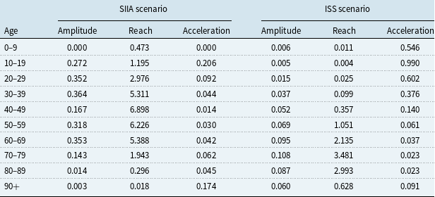
Table 1 shows the estimates of the amplitude $\alpha \!\left( x \right)$
, reach
$\alpha \!\left( x \right)$
, reach $\rho \!\left( x \right)$
, and acceleration
$\rho \!\left( x \right)$
, and acceleration $\pi \!\left( {{\rm{t}},x} \right)$
parameters by age groups in the first wave:
$\pi \!\left( {{\rm{t}},x} \right)$
parameters by age groups in the first wave:
Table 1. Estimation of amplitude, reach and acceleration in the first wave.

In Table 1, by observing the amplitude parameter $\alpha \!\left( x \right)$
, we see that there is a notable difference in the proportion of deaths by ages. In particular, in the scenario based on the SIIA data, a higher Covid-19-related mortality emerges for all age groups, except ages 0–9 (due to the absence of hospitalised Covid-19 of that age group in the dataset). This suggests that, for the same age, hospitalised persons have a greater risk of death from Covid-19 than other infected persons. Furthermore, deaths are concentrated in the middle ages (between 30 and 59 years) for the SIIA scenario and for the most advanced ages (between 70 and 89 years) for the ISS one.
$\alpha \!\left( x \right)$
, we see that there is a notable difference in the proportion of deaths by ages. In particular, in the scenario based on the SIIA data, a higher Covid-19-related mortality emerges for all age groups, except ages 0–9 (due to the absence of hospitalised Covid-19 of that age group in the dataset). This suggests that, for the same age, hospitalised persons have a greater risk of death from Covid-19 than other infected persons. Furthermore, deaths are concentrated in the middle ages (between 30 and 59 years) for the SIIA scenario and for the most advanced ages (between 70 and 89 years) for the ISS one.
Also, with regard to the reach parameter $\rho \!\left( x \right)$
, the two scenarios differ considerably. In particular, in the scenario based on the SIIA data, the expected loss of years of life is more severe in the middle ages, with a maximum of 5 years lost on average for ages between 50 and 59 years and, although not null, the loss is more limited for the advanced ages. In contrast, for the ISS scenario, it is the ages over 60 who are most penalised by the reduction in life expectancy. This result is also attributable to the different composition of the populations analysed, noting, with respect to the amplitude, that the population of those hospitalised by Covid-19 is more frail and in particular in the middle ages, 40–79.
$\rho \!\left( x \right)$
, the two scenarios differ considerably. In particular, in the scenario based on the SIIA data, the expected loss of years of life is more severe in the middle ages, with a maximum of 5 years lost on average for ages between 50 and 59 years and, although not null, the loss is more limited for the advanced ages. In contrast, for the ISS scenario, it is the ages over 60 who are most penalised by the reduction in life expectancy. This result is also attributable to the different composition of the populations analysed, noting, with respect to the amplitude, that the population of those hospitalised by Covid-19 is more frail and in particular in the middle ages, 40–79.
For the values of $\pi$
(t, x), similar values are observed across the two scenarios, except at the younger ages, due to the fact that, in some age groups, no deaths were recorded for both scenarios. In any case, there is a greater acceleration of mortality in the younger ages, but a greater mortality level in the more advanced ages in absolute terms. This is due to the fact that mortality at low or middle age causes a greater loss in terms of life expectancy than in older ages.
$\pi$
(t, x), similar values are observed across the two scenarios, except at the younger ages, due to the fact that, in some age groups, no deaths were recorded for both scenarios. In any case, there is a greater acceleration of mortality in the younger ages, but a greater mortality level in the more advanced ages in absolute terms. This is due to the fact that mortality at low or middle age causes a greater loss in terms of life expectancy than in older ages.
Table 2 shows the estimation of amplitude $\alpha \!\left( x \right)$
, reach
$\alpha \!\left( x \right)$
, reach $\rho \!\left( x \right)$
, and acceleration
$\rho \!\left( x \right)$
, and acceleration $\pi \!\left( {{\rm{t}},x} \right)$
parameters by age groups in the second wave:
$\pi \!\left( {{\rm{t}},x} \right)$
parameters by age groups in the second wave:
Table 2. Estimation of amplitude, reach and acceleration in the second wave.
The amplitude parameter $\alpha \!\left( x \right)$
is higher for ages up to 69 in the SIIA scenario than in the ISS scenario, and it is similar for ages 70–90 and lower for the 90+ scenario. In other words, the SIIA scenario places more emphasis on ages that are not extreme than the ISS scenario. This aspect, as in the previous case, depends on the hospitalisations on which the data from which the SIIA scenario is based.
$\alpha \!\left( x \right)$
is higher for ages up to 69 in the SIIA scenario than in the ISS scenario, and it is similar for ages 70–90 and lower for the 90+ scenario. In other words, the SIIA scenario places more emphasis on ages that are not extreme than the ISS scenario. This aspect, as in the previous case, depends on the hospitalisations on which the data from which the SIIA scenario is based.
The reach parameter $\rho \!\left( x \right)$
is higher for ages up to 69 years in the SIIA scenario than in the ISS scenario, with a loss of life expectancy up to around 5–7 years in the age groups between 30 and 69 which, in this case, are the most affected classes. In contrast, in the ISS scenario, the most affected age groups are those between 60 and 89 years, with a loss of life expectancy between 2 and 3 years approximately. This difference depends not only on the distribution by different age of the two databases on which the scenarios are based, but also on the different distributions of frailties. Thus, in the SIIA database, mostly fragile subjects are present and therefore are more exposed to premature death than in the ISS database that relates to the whole population, and therefore also includes people without co-morbidities who have an experience of Covid-19 with no or few symptoms. The greater frailty leads to a greater loss of years of life expectancy due to the effects of Covid-19.
$\rho \!\left( x \right)$
is higher for ages up to 69 years in the SIIA scenario than in the ISS scenario, with a loss of life expectancy up to around 5–7 years in the age groups between 30 and 69 which, in this case, are the most affected classes. In contrast, in the ISS scenario, the most affected age groups are those between 60 and 89 years, with a loss of life expectancy between 2 and 3 years approximately. This difference depends not only on the distribution by different age of the two databases on which the scenarios are based, but also on the different distributions of frailties. Thus, in the SIIA database, mostly fragile subjects are present and therefore are more exposed to premature death than in the ISS database that relates to the whole population, and therefore also includes people without co-morbidities who have an experience of Covid-19 with no or few symptoms. The greater frailty leads to a greater loss of years of life expectancy due to the effects of Covid-19.
The acceleration parameter $\pi \!\left( {{\rm{t}},x} \right)$
based on the SIIA and the ISS scenarios differ according to the age group.
$\pi \!\left( {{\rm{t}},x} \right)$
based on the SIIA and the ISS scenarios differ according to the age group. $\pi \!\left( {{\rm{t}},x} \right)$
, which depends on amplitude and reach, also differs significantly in the two scenarios. In particular, if it is observed that the acceleration increases with increasing age, an aspect that depends on the base scenario (and therefore on the mortality table on which the estimate is based), the ISS scenario tends to overestimate the acceleration due to Covid-19 compared to the SIIA scenario for all ages. This aspect underlines the importance of distinguishing between frail and non-frail populations in the context of an analysis of the effects of Covid-19 mortality.
$\pi \!\left( {{\rm{t}},x} \right)$
, which depends on amplitude and reach, also differs significantly in the two scenarios. In particular, if it is observed that the acceleration increases with increasing age, an aspect that depends on the base scenario (and therefore on the mortality table on which the estimate is based), the ISS scenario tends to overestimate the acceleration due to Covid-19 compared to the SIIA scenario for all ages. This aspect underlines the importance of distinguishing between frail and non-frail populations in the context of an analysis of the effects of Covid-19 mortality.
Since life expectancy also depends on the age of individuals, in order to isolate the effects of the pandemic on the loss of years of life, we consider a relative measure of reach, which is given by the ratio between the number of years of life expectancy lost and attributable to Covid-19 and the life expectancy for the same year calculated with the Renshaw–Haberman model, and calculated in the absence of mortality data from Covid-19. Table 3 compares the results of the two available databases (ISS and SIIA) for the two waves.
Table 3. Estimation relative reach for the first and the second wave.

As shown in Table 3, the relative reach differs according to the dataset and the wave considered. In particular, for the SIIA scenario, we can observe a greater relative loss of life expectancy for the age groups from 70, with over the 20% of total life expectancy lost for ages 70–89; while for the second wave, the effect at the older ages is reduced. In any case, the loss of life expectancy remains negligible for ages up to 29. In this sense, we can see a difference in mortality between the first and second waves, with the latter affecting the middle ages to a greater extent than the first wave, in which the mortality impact seems to be focussed on the older age groups. The ISS scenario is even more optimistic for the younger ages, with a relative loss of years of life expectancy lower than 1% up to age 49. We also observe that between the first and the second waves there are no marked differences in terms of relative loss of life expectancy. As also observed in Tables 1 and 2, the differences between the two scenarios show that the subpopulation of hospitalised patients has different demographic characteristics compared to the total population infected with Covid-19. In fact, the results for the subpopulation of the hospitalized show that individuals in the middle age groups are more sensitive to mortality and, consequently, to the loss of years of life expectancy and this is even more evident during the second wave, which affected a wider portion of the population.
Projections
In order to compute the acceleration $\;A\!\left( {x,t} \right)$
as in formula (2),
$\;A\!\left( {x,t} \right)$
as in formula (2), $q\!\left( {x,t} \right)$
is obtained by the baseline model, measured by Renshaw–Haberman model (from herein RH – see Renshaw and Haberman, Reference Renshaw and Haberman2003).
$q\!\left( {x,t} \right)$
is obtained by the baseline model, measured by Renshaw–Haberman model (from herein RH – see Renshaw and Haberman, Reference Renshaw and Haberman2003). $SIRf\!\left( {x,t} \right)$
is measured by an implied frailty formula, smoothed by age using a p-spline function.
$SIRf\!\left( {x,t} \right)$
is measured by an implied frailty formula, smoothed by age using a p-spline function. $\lambda \!\left( {x,t} \right)$
is measured by a Gompertz dynamic model as defined by Harvey and Kattuman (Reference Harvey and Kattuman2020).
$\lambda \!\left( {x,t} \right)$
is measured by a Gompertz dynamic model as defined by Harvey and Kattuman (Reference Harvey and Kattuman2020).
 \begin{align*}q\!\left( {x,t} \right)\end{align*}
The mortality data for the Italian population are downloaded from the Human Mortality Database ranging from 1950 to 2017, aggregated by gender for all the ages from 0 to 100. Projection of all causes mortality rates at age x and time t is used as in the baseline scenario. The choice of stochastic mortality model will need to accommodate an analysis of mortality by cohort for the application to insurance premiums and, as a consequence, a cohort analysis of the effect on mortality of the pandemic shocks is obtained using the multiplicative factors of formula (2).
To choose the best stochastic mortality model, a comparison is made of the goodness of fit of 4 widely used models using the AIC and BIC indices to the HMD data for 1950–2017. The models chosen come from the Lee-Carter family (basic Lee-Carter, Renshaw-Haberman, APC) and the Cairns-Blake-Dowd family (M7, see Cairns et al. paper, 2009).
The Lee Carter family models represent a well-known paradigm in the actuarial literature and practice devoted to the stochastic mortality models for the description of the future mortality evolution.
In particular, several researchers on the topic have shown good fitting and the best results in prediction in the case of the Italian population ranging from 0 to 100 years collected from 1950 to nowadays. For instance, we mention Brouhns et al. (Reference Brouhns, Denuit and Vermunt2002), D’Amato et al. (Reference D’Amato, Di Lorenzo, Russolillo and Sibillo2011a,b, 2012), Danesi et al. (Reference Danesi, Haberman and Millossovich2015) and so on.
As shown by Table 4, the model with the best goodness of fitting among those considered is RH.
 \begin{align*}\lambda \!\left( {x,t} \right)\end{align*}
Table 4. Baseline mortality models comparison.

In order to choose the best predictor for infection rate, we estimate a Gompertz dynamic model as defined by Harvey and Kattuman (Reference Harvey and Kattuman2020). This model is based on a dynamic linear model that is widely used for time series data to model time-varying parameters. As shown by the authors, the model of new infection growth rate, that is log(y t – y t -1) is modelled as a random walk with drift and an exogenous trend. Further details about this approach are described in Appendix.
In order to implement the estimation, we use the dlm library in R. To do this, we define a two-state model, where the first state equals its previous value plus the second state plus the normal random walk step and the second state estimates the trend.
Figure 1 shows the in-sample forecasting of the model:
As shown in Figure 1, the model can fit both the first and the second waves, unlike traditional ARIMA or trend interpolation techniques, for which experiments demonstrate that the first wave makes the fitting worse and the use of a unique model is not adequate for the entire time series.

Figure 1 Dynamic Gompertz model in-sample forecasting.
Figure 2 shows out-of-sample forecasting for this model at a time lag of 10 steps ahead, that corresponds to 10 days.

Figure 2 Dynamic Gompertz model out-of sample forecasting.
As Figure 2 shows, the forecasts follow the growing trend of the latest observation. This is a positive feature for this class of model but, like the others, it provides a reliable forecast only for short-term horizons. In Harvey and Kattuman (Reference Harvey and Kattuman2020), the “second wave” estimation is based on the change of trend parameter $\gamma$
t, while the forecast function of the routine is based on the latest value of
$\gamma$
t, while the forecast function of the routine is based on the latest value of $\gamma$
t
.
$\gamma$
t
.
 \begin{align*}SIRf\!\left( {x,t} \right)\end{align*}
Implied relative frailty is calculated using observed data. In equation (2), we note that all the elements, except for relative frailty, are observed. In particular, for the all-causes mortality rate, we use the data from the all causes of deaths ISTAT daily mortality database, which contains the daily deaths by age group at municipality level from the 1st January to 31st December 2020. The Covid-19 mortality rate is available from ISS monitoring reports, observing the cumulated deaths for age group by Covid-19 each week. In this case, we consider the data of the last week of 2020. Finally, the infection rate is estimated from the Protezione Civile’s time series (Dipartimento della Protezione Civile, 2020), which reports the number of new daily infected aggregated for all ages. In order to obtain the infection rate, we use the log difference of the series. Table 5 shows estimated implied frailty based on the Italian data for the last week of 2020:
Table 5. Implied frailty.

As shown in Table 5, implied frailty shows an increasing value up to 70–79 age class and then it decreases. In order to improve the estimation results and obtain a less peaked function of age, we use a p-spline smoother for the implied frailty estimation. The smoothing is applied using the all-causes of deaths by age as an offset and the results are shown in Figure 3:

Figure 3 Frailty estimated using observed data and smoothing based on all causes of deaths by age.
Figure 3 shows that smoothing allows us to obtain a functional form for implied frailty similar to a logistic curve. Figure 4 shows the Covid-19 mortality rates estimated using the smoothed frailty function:

Figure 4 Covid-19 mortality rates estimated using smoothed frailty and implied frailty.
Figure 4 shows that the Covid-19 mortality rates are quite similar using smoothed and implied frailty values. For the age groups 60–69, 70–79 and 80–89, the smoothed frailty estimates give slightly higher mortality rate estimates.
 \begin{align*}A\!\left( {x,t} \right)\end{align*}
In order to obtain a forecast of acceleration, we use the Renshaw-Haberman stochastic mortality model as a baseline for all causes of death mortality rates in the absence of acceleration effects and we use equation (2).
Figures 5–8 shows the estimated numbers of Covid-19 deaths by age for two fixed years, that is 2021 and 2041, in order to observe the effects of $A\!\left( {x,t} \right)$
in the short-term and long-term and by year at two fixed ages, that is 50 and 90, in order to observe the effects of
$A\!\left( {x,t} \right)$
in the short-term and long-term and by year at two fixed ages, that is 50 and 90, in order to observe the effects of $A\!\left( {x,t} \right)$
on middle and extreme ages.
$A\!\left( {x,t} \right)$
on middle and extreme ages.

Figure 5 Projection of baseline and accelerated deaths by age for 2021.

Figure 6 Projection of baseline and accelerated deaths by age for 2041.

Figure 7 Projection of baseline and accelerated deaths by years for age 50.

Figure 8 Projection of baseline and accelerated deaths by years for age 90.
As can we observe from Figures 5–8, the effect of Covid-19 on mortality rates is a short-term phenomenon. Although it affects the most frail part of the population, there appears to be no long-term repercussions in terms of premature deaths. Covid-19 mortality has some persistence in the very old population compared with the younger population; however, the impact on mortality is marginal with respect to the wider longevity effects experienced by the population.
Comparing the first and the second waves, we observe – alongside an age effect – a frailty effect on mortality caused by Covid-19, related to the hospitalised sub-population. The effect is more evident in the second wave, where the access to medical treatment in Italy was open to people at all ages.
Estimation of projections of Covid-19 mortality rates allows us to evaluate the effects by age and time of Covid-19 on mortality rates. As observed, although effects persist for some higher ages, mortality is not affected by the Covid-19 pandemic in the long term.
The impact on traditional insurance contracts
In order to assess the impact of Covid-19 mortality acceleration on the insurance market, we compared the premiums of some of the main (non-participating) life contracts using survival probabilities from the baseline and accelerated cases.
In particular, we consider, for persons aged x = 40, 50, 60, 70 and t = 2022:
-
• An immediate annuity with a technical interest rate of 1% and an annual payment of 5,000;
-
• A term insurance with a technical interest rate of 4% and an insured amount of 25,000 for 10, 20 and 30 years;
-
• A pure endowment with a technical interest rate of 2% and an insured amount of 25,000 for 10, 20 and 30 years.
For each contract, we define:
-
• The single premium;
-
• The insured amount with a single premium equal to
$\unicode{x20AC}$
10,000; -
• The premium adjustment
${\vartheta _A}$
; -
• The acceleration insurance ratio (AIR).


The results are shown in Tables 6–9:
Table 6. Life insurance contracts comparison x = 40.

Table 7. Life insurance contracts comparison x = 50.

Table 8. Life insurance contracts comparison x = 60.

Table 9. Life insurance contracts comparison x = 70.

As shown in Table 6, for an individual aged 40, there are some differences in the single premium, and these depend on the kind of contract. In particular, for the immediate annuity, the adjusted premium is lower by about 1,134 euros than the baseline premium, since the probability of survival at the same age decreases as a result of Covid-19. For the same reason, the premium of the pure endowment also decreases considering the acceleration and it is lower for longer maturity periods, that is with a difference of 28.76, 50.9 and 62.83 euros for 10, 20 and 30 years, respectively. In contrast, for the term insurance, the reduction of the survival probabilities due to mortality acceleration leads to an increase in the premium. So, the premium adjustment is negative in the case of life insurance and positive in the case of contracts providing survival benefits (like annuities and pure endowments). Furthermore, the longer is the maturity period of the contract, the greater is the acceleration in absolute terms, with increases of 28.46, 50.76 and 65.05 euros for 10, 20 and 30 years. In contrast, in relative terms, there is a decrease in AIR by duration of the contract for term insurance, with differences of 20.55% for 10 years, 10.68% for 20 years and 5.89% for 30 years, and for the pure endowment with differences of −0.14%, −0.31% and −0.51% for 10, 20 and 30 years respectively.
As shown in Table 7, for an individual aged 50, the differences also depend on the contract. As previously observed, for the annuity and pure endowment, the single premium is lower if the acceleration is considered, with a lower premium of 1023.72 euros for annuity, and for the pure endowment the longer the maturity period the greater is the difference with −34.32, −55.75 and −63.31 euros for 10, 20 and 30 years. In contrast, for the term insurance, the premium is higher and increases as the maturity period increases, that is 34.01 euros for 10 years, 56.68 for 20 years and 68.95 for 30 years. However, as previously observed, AIR reduces as the duration of contract increases for the term insurance, moving from 6.77% for 10 years to 3.93% for 20 years and 2.31% for 30 years, and for the pure endowment, moving from −0.17% for 10 years to −0.37% for 20 years to −0.63% for 30 years.
As shown in Table 8, for an individual aged 60, there are similar results. In particular, for the annuity and pure endowment, there is a decrease in the premium of 986.55 euros and 37.14, 57.61 and 76.21 euros, depending on the duration, and an increase in the term insurance premium of 36.95, 59.68 and 82.38 euros as the duration increases. As already noted, in relative terms, there is an inverse relationship with the duration of the contract, with an AIR of 2.59%, 1.58% and 1.12% for 10, 20 and 30 years, respectively, for the term insurance and an AIR of −0.20%, −0.46% and −1.54% for 10, 20 and 30 years for the pure endowment.
As shown in Table 9, for an individual aged 70, there are similar results. For the annuity and pure endowment, the premium is lower by 925.85 euros and of 43.68 euros for 10 years, 91.06 euros for 20 years and 87.60 euros for 30 years with the use of accelerated survival probabilities. In contrast, for term insurance, if the acceleration is considered, the premium is higher by 43.68 euros for 10 years and 91.06 for 20 year. The AIR is lower both for pure endowment and term insurance, by −0.26% and −1.34% and 1.16% and 0.97%, respectively.
Observing Tables 6–9 individually allows us to make an analysis by cohorts, observing how a different mortality table affects the insurance contracts. Also, comparing the results of Tables 6–9 by age allows us to compare different specific ages. The relationship between age and the acceleration of mortality has an impact on the insurance contracts, which can be separated as the effect of the extra premium for age due to the pandemic increase in mortality and the age effect on the premium. As can be observed from the tables, if only the absolute difference, that is the premium adjustment ${\vartheta _A}$
, is considered, that the premium increases in absolute values as the age increases for the term insurance and pure endowment with equal durations and it decreases for the immediate annuity. In contrast, considering the AIR, the relative difference increases for the annuity and pure endowment, and it decreases for the term insurance. The reason is that the effects of indirect acceleration, due to the pandemic effects on mortality, are smaller than the effect of direct acceleration, due to increasing age (i.e. normal ageing). In this sense, although an extra premium is observed, being negative for the pure endowment and annuity contracts and positive for the term insurance contracts, the difference is smaller than the difference arising from increases in the insured person’s age. For this reason, there is an increase in the difference in the age premium for annuity and pure endowment and a decrease in term insurance. This result seems to suggest that the impact of the pandemic on the insurance market, although it is not zero, would nevertheless be modest.
${\vartheta _A}$
, is considered, that the premium increases in absolute values as the age increases for the term insurance and pure endowment with equal durations and it decreases for the immediate annuity. In contrast, considering the AIR, the relative difference increases for the annuity and pure endowment, and it decreases for the term insurance. The reason is that the effects of indirect acceleration, due to the pandemic effects on mortality, are smaller than the effect of direct acceleration, due to increasing age (i.e. normal ageing). In this sense, although an extra premium is observed, being negative for the pure endowment and annuity contracts and positive for the term insurance contracts, the difference is smaller than the difference arising from increases in the insured person’s age. For this reason, there is an increase in the difference in the age premium for annuity and pure endowment and a decrease in term insurance. This result seems to suggest that the impact of the pandemic on the insurance market, although it is not zero, would nevertheless be modest.
In brief: from the data to the main results
We start to study the being the first European country severely hit by Covid-19 infection. Thanks to the availability of clinical data relating to Italian hospitals and medical centres, we observe that the mortality “accelerates” in the group of population with co-morbidities at Covid-19 diagnosis.
We considered separately the subpopulation of hospitalised patients and the total population infected with Covid-19. We can observe a notable difference in the age distribution of deaths. In fact, if we consider only those who have a severe course of the disease, we observe a higher mortality in the middle or high but not extreme ages, while, on the contrary, if we consider the totality of the population, the effects of mortality due to Covid-19 seem to relate more to the extreme ages. We can argue, therefore, that mortality due to Covid-19 mainly depends both on the age of the infected person and on his clinical conditions.
In particular, we show that the mortality shock is greater for the older population groups and for individuals who present co-morbidities, which aggravate their state of health in the case of infection. However, the evidence points to a non-persistent shock, with the acceleration tending to be softened in the long run. Finally, we evaluate the impact of the Covid-19 acceleration on the insurance market. We point out that although there is an impact of the acceleration on the premium, it is still low compared with other factors that contribute to the determination of the premium. In line with Harris (2021), we can see small adjustments in the life insurance offering that correspond to increases in mortality risk perceived from insurers as modest in the short run.
5. Concluding Remarks
In this paper, we have assessed the excess mortality due to the Covid-19 pandemic for the Italian case. Firstly, we estimate the acceleration of the mortality through the observed data, comparing the total population with a subpopulation who are more exposed to mortality risks, that is a hospitalised population, to highlight the presence of a non-uniform mortality shock in the population. Accordingly, we propose an acceleration model that allows the future acceleration to be projected as a function of the trend of infections and a frailty parameter, estimated as an implicit parameter that depends on age. In this way, it is possible to project the acceleration of mortality and observe the possible effects by age and time. Finally, we evaluate the impact of the acceleration in the insurance market, comparing the premiums of some basic life insurance contracts. In particular, we observe that the mortality shock is greater for the older population groups and for individuals who present co-morbidities which aggravate their state of health in the case of infection. However, the evidence points to a non-persistent shock, with the acceleration tending to be softened in the long run.
In terms of the impact on the insurance market, it is noted that, although there is an impact of the acceleration on the premium, it is still low compared to other factors that contribute to the determination of the premium. Further research will be addressed in order to assess how the temporarily stressed mortality rates change the post-Covid-19 mortality rates and affect longevity trends and to develop metrics to measure population frailty in terms of health status by age.
Appendix
The Gompertz Dynamic Model proposed by Harvey & Kattuman (Reference Harvey and Kattuman2020) consists of an extension to a Linear Dynamic Model which allows us to construct a time-varying parametric model for a non-linear curve, in this case a logistic curve, which is defined by Gompertz function. This approach may be used to model the evolution of the infection of a pandemic.
Let us consider a Gompertz function, where the cumulative function to t -1is the response variable and the positive change is ${y_t} = \;\Delta {Y_t} = {Y_t} - {Y_{t - 1}}$
:
${y_t} = \;\Delta {Y_t} = {Y_t} - {Y_{t - 1}}$
:
 \begin{align}{\rm{ln}}\;{y_t} = \rho \;ln\;{Y_{t - 1}} + {\rm{\delta }} - {\rm{\gamma }}t\; + \;{\varepsilon _{\rm{t}}},\;\rho \ge 1,\;t\; = \;2, \ldots ,\;T\end{align}
where ${\varepsilon _{\rm{t}}}$
is independent and identically distributed error term with zero mean and
${\varepsilon _{\rm{t}}}$
is independent and identically distributed error term with zero mean and $\sigma _\varepsilon ^2$
variance. Subtracting
$\sigma _\varepsilon ^2$
variance. Subtracting ${Y_{t - 1}}$
from both sides, a simple time trend regression is obtained:
${Y_{t - 1}}$
from both sides, a simple time trend regression is obtained:
 \begin{align}{\rm{ln}}\;{g_t} = {\rm{\delta }} - {\rm{\gamma }}t\; + \;{\varepsilon _{\rm{t}}},\;t\; = \;2, \ldots ,\;T\end{align}
If a stochastic trend into formula (A.2) is introduced, we obtain a Gompertz Dynamic Model:
 \begin{align}{\rm{ln}}\;{g_t} = {\delta _t} + \;{\varepsilon _t},\;\;{\varepsilon _t}\sim IID\!\left( {0,\;\sigma _\varepsilon ^2} \right)\end{align}
 \begin{align*}{\delta _t} = {\delta _{t - 1}} - {{\rm{\gamma }}_{t - 1}} + \;{\eta _{\rm{t}}},\;\;{\eta _{\rm{t}}}\sim IID\!\left( {0,\;\sigma _\eta ^2} \right)\end{align*}
 \begin{align*}{{\rm{\gamma }}_t} = {{\rm{\gamma }}_{t - 1}} + \;{\zeta _{\rm{t}}},\;\;{\zeta _{\rm{t}}}\sim IID\!\left( {0,\;\sigma _\zeta ^2} \right)\end{align*}
with independent $\;{\varepsilon _t}$
,
$\;{\varepsilon _t}$
, ${\eta _{\rm{t}}}$
and
${\eta _{\rm{t}}}$
and ${\zeta _{\rm{t}}}$
. Formula (A.3) shows that the model is composed of an exogenous trend
${\zeta _{\rm{t}}}$
. Formula (A.3) shows that the model is composed of an exogenous trend ${\rm{ln}}\;{g_t}$
, where the parameter
${\rm{ln}}\;{g_t}$
, where the parameter ${\delta _t}$
is a random walk with drift minus a lagged parameter
${\delta _t}$
is a random walk with drift minus a lagged parameter ${{\rm{\gamma }}_{t - 1}}$
which itself is modelled as a random walk. All the parameters are estimated using MLE.
${{\rm{\gamma }}_{t - 1}}$
which itself is modelled as a random walk. All the parameters are estimated using MLE.


 Open access