


1. Introduction
Due to increased economic growth in recent years, cities in the United States are facing yet another wave of sprawl, with development converting hinterlands surrounding cities to urban uses (Sorensen et al. Reference Sorensen, Freedgood, Dempsey and Theobald2018). Cities in regions with embedded beliefs that land development rights should not be restricted by governmental organizations find themselves with few legal tools to control the direction and rate of land conversion (Pincetl Reference Pincetl2006). At the same time, urban communities are experiencing pressure to approach development in a planned, sustainable manner so that nearby lands, including forestland, pastureland, and cropland, can be preserved to maintain ecosystem services such as offsetting greenhouse gas (GHG) emissions in the face of climate change (Reid and Satterthwaite Reference Reid and Satterthwaite2007; de Zeeuw and Dubbeling Reference de Zeeuw and Dubbeling2009; Condon et al. Reference Condon, Mullinix, Fallick and Harcourt2010; Dubbeling and de Zeeuw Reference Dubbeling and de Zeeuw2011; Hellwinckel et al. Reference Hellwinckel, Menard, Wilson, Howell, Parkman and Haugen2014).
A common conservation strategy is to establish protected areas through land acquisition using conservation contracts, such as fee simple acquisitions and conservation easements (Land Trust Alliance 2019). In establishing protected areas through acquisition, the non-market values of those areas to communities are typically acknowledged, and valuations have been approached through estimating communities’ willingness to pay (WTP) for the programs using survey analysis (Cho, Newman, and Bowker Reference Cho, Newman and Bowker2005; Hemby Reference Hemby2016; Vizek and Nielsen-Pincus Reference Vizek and Nielsen-Pincus2017). Those studies typically estimate WTP for hypothetical or factual programs to assess potential support and values to the communities. Although this approach has provided evidence of demand for land preservation, potentially high levels of uncertainty regarding benefits and costs of protected areas have been mostly ignored in the literature. Economic growth fluctuations are a vital source of uncertainty related to conservation costs because the opportunity cost of holding land depends on fluctuations in the returns from competing land uses such as urban development (Schatzki Reference Schatzki2003; Verick and Islam Reference Verick and Islam2010). For example, the opportunity cost of deforestation for urbanization fluctuates depending on real estate market conditions and thus affects the performance of conservation investments (Cho et al. Reference Cho, Lee, Roberts, Edward and Armsworth2018; Cho and Sharma Reference Cho and Sharma2019).
A branch of literature deals with the uncertainty associated with conservation benefits in targeting conservation investments (Williams et al. Reference Williams, Hannah, Andelman, Midgley, Araújo, Hughes, Manne, Martinez-Meyer and Pearson2005; Pressey et al. Reference Pressey, Cabeza, Watts, Cowling and Wilson2007; Heller and Zavaleta Reference Heller and Zavaleta2009; Hodgson et al. Reference Hodgson, Thomas, Wintle and Moilanen2009; Carvalho et al. Reference Carvalho, Brito, Crespo, Watts and Possingham2011; Armsworth et al. Reference Armsworth, Larson, Jackson, Sax, Simonin, Blossey, Green, Klein, Lester, Ricketts and Runge2015; Albers et al. Reference Albers, Busby, Hamaide, Ando and Polasky2016). Many of those studies focus on the influence of climate uncertainty on the benefits of conservation investments that affect the spatial targeting of investments (Hultman Reference Hultman2006; Ando et al. Reference Ando, Fraterrigo, Guntenspergen, Howlader, Mallory, Olker and Stickley2018; Runting et al. Reference Runting, Beyer, Dujardin, Lovelock, Bryan and Rhodes2018). For example, the risk-diversification strategy of Markowitz (Reference Markowitz1952) from the finance perspective is suggested as a way to incorporate future climate uncertainty related to ecological outcomes (i.e., program benefits) in allocating conservation investments (Halpern et al. Reference Halpern, White, Lester, Costello and Gaines2011; Ando and Mallory Reference Ando and Mallory2012; Dunkel and Weber Reference Dunkel and Weber2012; Hoekstra Reference Hoekstra2012; Mallory and Ando Reference Mallory and Ando2014; Shah et al. Reference Shah, Mallory, Ando and Guntenspergen2017).
Limited literature deals with the variation in costs and benefits under changing climatic or economic conditions for optimal spatial conservation investment decisions. For example, Mallory and Ando (Reference Mallory and Ando2014) utilized modern portfolio theory (MPT) to address fluctuations in both the ecological benefits and land values of potential conservation sites under uncertain future climate-change scenarios. The authors incorporated benefits and costs, which vary spatially across multiple scenarios, into the variance-covariance structure to generate a portfolio of conservation sites corresponding to an optimal mean-variance combination reflecting risk-return preference. Despite such efforts, few studies have focused on the impact of the risk derived from uncertainty in conservation costs associated with economic growth uncertainty and its implications for the spatial targeting of conservation and restoration investments. The risks associated with conservation costs, such as land acquisition costs, are mostly driven by persistent uncertainty in relevant land values, thus requiring their forecasting and incorporation into conservation investment decisions.
Incorporating uncertainty of economic growth into decisions related to protected area acquisition is critical to prioritizing spatial targets based on conservation return-on-investment (ROI), commonly quantified by dividing a numerical measure of the conservation benefit by an historic estimate of the acquisition cost (e.g., Murdoch et al. Reference Murdoch, Polasky, Wilson, Possingham, Kareiva and Shaw2007; Goldstein Pejchar, and Daily Reference Goldstein, Pejchar and Daily2008; Wilson et al. Reference Wilson, Lulow, Burger, Fang, Andersen, Olson, O’Connell and McBride2011; Withey et al. Reference Withey, Lawler, Polasky, Plantinga, Nelson, Kareiva, Wilsey, Schloss, Nogeire, Ruesch and Ramos2012; Kovacs et al. Reference Kovacs, Polasky, Nelson, Keeler, Pennington, Plantinga and Taff2013; Sutton and Armsworth Reference Sutton and Armsworth2014; Armsworth et al. Reference Armsworth, Jackson, Cho, Clark, Fargione, Iacona, Kim, Larson, Minney and Sutton2017; Cho et al. Reference Cho, Thiel, Armsworth and Sharma2019). Historic estimates of conservation ROI that ignore uncertainty of economic growth may mislead the spatial targeting of protected area acquisition.
Under the assumption that a conservation agency is interested in cost-efficient budget allocation, protected area acquisition from the agency's perspective is a riskier investment than short-term conservation investment, such as payments for ecosystem services, because the former is typically irreversible once implemented. Given the uncertainty in future economic growth, the possibility of spatially varying changes in costs and benefits that leads to spatially varying changes of ROI in the future is a potential risk to the conservation objective of spatially allocating a budget cost-efficiently. Hence, we recognize a critical need to balance risk and return in spatial targeting of protected areas for acquisition based on anticipated future economic growth conditions.
To fill the gap in the literature, we find spatially optimal budget allocations for acquiring protected areas to store carbon on forestland, pastureland, and cropland by balancing the risk and return from protection under three economic growth scenarios (i.e., strong, weak, moderate). In doing so, our study is the first to apply the risk of uncertain economic growth that affects the cost of protected area acquisition using real estate values at the parcel level, which is described in detail in Step 2 of the four-step procedure in the “Method and Data” section. This spatial resolution is required because achieving cost efficient outcomes relies on how finely a conservation agency can resolve spatial variation in costs and use this variation in applying the site-specific opportunity costs of supplying carbon storage. The findings from the empirical model provide a critical way to deal with the risk of uncertain economic growth that affects the cost of protected area acquisition for the purpose of preserving carbon storage in a local community, which has never been done before.
We focus on the spatial targeting of potential candidate areas and their optimal budget allocations with return measured by the total expected benefit of carbon storage and the risk measured by the variance of the total carbon storage benefit across uncertain future economic growth scenarios. The differences in forecasted acquisition costs and the resulting variability in conservation benefits across the future economic growth conditions comprise a conservation agency's risk associated with conservation investment.
We consider that a conservation agency wishing to implement land acquisitions in a local community under economic growth uncertainty has the options of either maximizing the expected benefit of carbon storage or maximizing the expected benefit for an acceptable variance level using the Mavrotas (Reference Mavrotas2009) multi-objective mathematical programming (MOMP) model. In the MOMP, the solution is the Pareto optimal one. We solve for several Pareto optimal budget allocations, each of which cannot be improved upon in terms of net benefits without increasing the variance. Under this premise, a completely risk-averse conservation agency would prefer widespread diversification of spatial investments to minimize the variance of benefits of carbon storage across the economic growth scenarios, while a risk-neutral agency would prefer spatial investments that maximize the expected benefit of carbon storage irrespective of the level of risk involved.
We find cluster-specific budget allocations (dollars invested in acquiring candidate areas from the clusters) based on optimal land acquisition decisions (hectares of candidate areas from the clusters) that represent Pareto-optimal solutions that maximize the total expected carbon storage (dollar values of the tons of carbon stored) at a given level of variance from the acquired clusters primarily dictated by the forecasted acquisition cost (dollar per hectare) and associated available carbon storage (tons per hectare) in eligible clusters. Our framework of a cluster-specific budget distribution implicitly assumes that determining the budget distribution for larger geographic areas, like our clusters, is a necessary first step prior to more micro-level funding allocation decisions, i.e. parcel-level decisions.
A conservation agency determining optimal clusters for a given combination of optimized risk and return can either implement MOMP or MPT to achieve the objectives. Noticeable differences exist between these approaches in the ways objectives are defined and addressed. First, our MOMP approach maximizes the total expected benefit of carbon storage at a given variance of total carbon storage and a specified expected budget constraint, while the MPT approach maximizes the portfolio expected ROI for a given portfolio variance. Second, the objective function for our MOMP approach is driven by hectares of clusters, whereas it is guided by spatial portfolio weights in the MPT approach. Third, the total expected benefit of carbon storage in our MOMP approach is the probability weighted sum of the benefits of total carbon storage across the economic growth scenarios, whereas the portfolio expected ROI in the MPT approach is the portfolio weighted sum of the expected ROIs of the clusters. Fourth, the variance in our MOMP approach is the variance of the benefit of total carbon storage across the economic growth scenarios, while the portfolio variance in the MPT approach is a composite term consisting of portfolio weights and a variance-covariance structure of cluster ROIs across economic growth scenarios.
Because of the MOMP approach's inability to take advantage of the full benefit of diversification by addressing the variance-covariance structure across clusters, optimal spatial targeting is potentially riskier than targeting based on the MPT. For example, the carbon storage benefits could have the identical spatial variance but different combined response (covariance) across alternative economic growth scenarios. If a conservation agency is focusing on balancing the return and risk of conservation investment, the variance-covariance structure, rather than individual variances, would make cost-effective budget allocation. Thus, optimal spatial targeting based on the MOMP approach is potentially riskier than targeting based on criteria that account for their variance-covariance structures.
Despite the relative disadvantage against the MPT, the MOMP approach has a computational advantage. Specifically, in our analysis a smaller number of uncertain scenarios (i.e., observations per asset in MPT) than the number of eligible clusters (i.e., assets in MPT) results in a non-invertible, non-positive semi-definite variance-covariance matrix of assets’ ROIs across scenarios. The problem arises because the number of assets that can be used in truly optimized optimal portfolio analysis should not exceed the limit of N-1 where N is the number of scenarios. For example, Ando et al. (Reference Ando, Fraterrigo, Guntenspergen, Howlader, Mallory, Olker and Stickley2018) conducted optimal portfolio analysis by creating 24 subunits for the U.S. portion of the Prairie Pothole Region, 7 subregions for birds of the Eastern U.S., and 11 subregions for Southern Appalachian salamanders across 71, 8, and 12 climate scenarios, respectively, where the number of subunits (or assets) is smaller than the number of scenarios (or observations per subunit).
The MOMP approaches have been widely used in literature addressing conflicting economic and environmental objectives either under the assumption of perfect or imperfect knowledge of random economic and environmental variables. For example, Zakariazadeh, Jadid, and Siano (Reference Zakariazadeh, Jadid and Siano2014) applied a stochastic multi-objective assessment of the operational method in a high-penetration wind energy generation and distribution system by minimizing the total expected operational costs and emissions providing a continuum of Pareto-optimal solutions. Under deterministic assumptions, a bicriterion feedstock cost and GHG emission minimization objective is considered in Yu et al. (Reference Yu, Wang, English and Larson2014) for determining an optimal switchgrass supply system in Tennessee, whereas Zhong et al. (Reference Zhong, Yu, Larson, English, Fu and Calcagno2016) applied a multi-objective optimization model to determine the potential trade-offs among the objectives of minimizing feedstock cost, GHG emission, and soil erosion in the design of a sustainable switchgrass supply chain in Tennessee. Both of these studies found that the type of agricultural land converted for switchgrass production has a major influence on the economic and environmental performance of the supply chain with the opportunity costs of land-use conversion and the net change in soil carbon sequestration under feedstock production being the major drivers of a particular kind of land-use change. Conceptually different from the aforementioned studies, Cho and Sharma (Reference Cho and Sharma2019) applied a MOMP approach using a mean-variance framework in spatial targeting of conservation investment for forest-based carbon sequestration in the U.S. central and southern Appalachian region addressing the risk preferences of conservation agencies in terms of conservation costs (net opportunity costs of retaining forestland) under economic growth uncertainty.
Given our objectives and the previously mentioned computational constraint, we use the MOMP approach under economic growth uncertainty to generate Pareto-optimal expected budget allocations that maximize the expected total carbon storage benefit at a given level of variance. This approach not only addresses uncertain economic growth but also provides optimal solutions for the expected benefit of carbon storage and its variance in an effort to balance the return and risk of conservation investment in protected area acquisition with the preferences of conservation agencies. In using this approach, we assume present optimal land acquisition decisions are made based on the anticipated probabilities of occurrence of future economic growth scenarios and agency preferences.
In addition to the MOMP approach, we solve the problem with a single-objective stochastic optimization approach that assumes risk-neutrality and deterministic optimization approaches that assume perfect knowledge of future economic growth. Figure 1 provides a schematic representation of the objective functions, decision variables, assumptions about economic growth uncertainty, associated risks, and intended applicability of the optimization approaches.

Figure 1. Schematic Representation of Cluster-Level Optimization Approaches (Note: Bold Arrows and Boxes Indicate the Schematic Portion of the MOMP Approach)
We use five clusters of land in and around the urban areas of Knox County, TN, as a case study (see Figure 2). A local community, instead of a larger area, is used as a case study because local communities are under increasing pressure to adopt innovative strategies to increase or sustain carbon storage (Elmqvist et al. 2015; Miller Hauer, and Werner Reference Miller, Hauer and Werner2015; Andersson-Sköld et al. Reference Andersson-Sköld, Klingberg, Gunnarsson, Cullinane, Gustafsson, Hedblom, Knez, Lindberg, Sang, Pleijel and Thorsson2018). The clusters are chosen for having large tracts of undeveloped contiguous land. Knox County, TN, is an appropriate case study because it has experienced sustained economic growth coupled with growth in population and income that has brought about rapid changes in land use and created pressure for GHG mitigation in the face of climate change (Murray et al. Reference Murray, Fox, Harris, Kessler, Cunningham, Glenn, Jensen, Menard, English, Griffith, Hughes, Smith, Yu, Blair and McCoy2018). Although Knox County, TN, is chosen as a case study, the procedure used to solve the MOMP problem to generate spatially optimal expected budget allocations under economic growth uncertainty can be replicated for any area where the necessary data are available for modeling (see the next section for details about the needed datasets).

Figure 2. Candidate Clusters of Parcels (Clusters 1, 2, 3, 4, and 5) in Knox County, TN
2. Method and Data
To accomplish the objective, we employ a four-step procedure (see a schematic representation of the four steps in Figure 3), which is organized in four subsections.

Figure 3. Schematic Representation of the Four Steps to Accomplish the Objective
Step 1: Identify Potential Candidates for Protection
The first step entails identifying land areas that are potential candidates for protected area acquisition in Knox County, TN. We initially identify five clusters for targeting given firsthand expert knowledge about local conservation issues based on interviews with local planners and other community representatives. Within each cluster, we use the National Land Cover Database (NLCD 2006, 2011) to select forestland, pastureland, and cropland areas that are eligible for protected area acquisition to store carbon.
We group the NLCD classifications of deciduous forest, evergreen forest, and mixed forest as “forestland,” pasture/hay and grassland/herbaceous as “pastureland,” and cultivated cropland as “cropland.” Then, within each cluster all eligible lands for acquisition are identified in each 1 km2 area, and the shares of the land-use categories are calculated for each of those areas and averaged across the areas within each cluster to form cluster-specific shares of eligible lands. This procedure was performed using data from the 2006 and 2011 NLCD datasets, assuming strong and weak economic growth scenarios based on the historical economic status in those years, respectively. These average shares are later converted to aggregated areas within each cluster for each of the three land-use categories as the product of the shares and the total cluster area. By averaging the shares of the 1 km2 areas for each land use, we simultaneously average the carbon stored in tons per hectare for each aggregated land use in each cluster. The aggregated area within each cluster as well as the average carbon stored in tons per hectare for each aggregated land use in each cluster for the moderate growth scenario is then assumed as the average value of the strong and weak economic growth scenarios. The area-weighted average of historic carbon stored within each cluster is later converted to scenario-specific U.S. dollar values using the U.S. Environmental Protection Agency (EPA)'s social cost of carbon (SCC), which is the value of avoided damage or the marginal cost of emission abatement, as benefit estimates.
Step 2: Forecast Acquisition Cost
In this step, we forecast (1) acquisition cost per hectare for each of the five clusters for each economic growth scenario, and (2) median housing values at the census-block group (CBG) level. Forecast of acquisition costs are based on 2018 average assessed land values and total housing values of the parcels that represent eligible lands for acquisition. We consider four parcel-level land-use classifications (i.e. agriculture/forestry/vacant, private recreation, right of way/open space, and rural residential) as lands (see Figure 2) that are potential candidates for carbon storage acquisition, because those areas are mostly undeveloped lands that can capture and store carbon in greater amounts than can the other land-use classifications (e.g., single and multi-family residential, and commercial).
We assume future residential property value as the leading indicator of the future value of the eligible parcels since the candidate parcel clusters are in or around urban communities within Knox County, TN, and their real estate values are dictated by residential property values. Under this assumption, we first develop an autoregressive distributed lag (ARDL) model at the CBG level using 1990–2016 data in which the median value of owner-occupied housing units (or median housing value) is regressed on three explanatory variables: unemployment rate, housing vacancy rate, and real mortgage rate. The latter is calculated as the nominal 30-year fixed rate (Federal Reserve Bank of St. Louis 2018) minus inflation (U.S. Bureau of Labor Statistics 2018). Annual median housing value data at the CBG level are only available for the years corresponding to the decennial U.S. Censuses in 1990 and 2000 (U.S. Census Bureau 1990, 2010). The 1990 data are used as the baseline year in estimating median housing values from 1991 to 1999 for each CBG. Median housing values are estimated by multiplying the previous year's housing value by the ratio of the current year's inflation-adjusted housing price index (HPI) to the previous year's HPI. Similarly, the median housing values from 2001 to 2016 are estimated using 2000 Census data and HPI data for 2001–2016.
Next, we apply average values of the three explanatory variables during the 1998–2006 and 2007–2012 periods as baselines for strong and weak economic growth scenarios, as those years loosely match with the corresponding growth cycle. Then we apply the future values of the independent variables to the ARDL model to forecast median housing value for each CBG in 2046 for the economic growth scenarios. The year 2046 as a future forecast year is a relatively ad hoc choice, because it is far enough in the future but not too far from the present. Any alternative future year meeting this criterion could be chosen without affecting the findings and general conclusions of our study. The average values for the three explanatory variables during the 1998–2006 and 2007–2012 periods are used to simulate future conditions for the strong and weak economic growth scenarios, respectively.
The 1990–2016 CBG data for the explanatory variables are obtained from U.S. Bureau of Labor Statistics (2018) and U.S. Census Bureau (2018). See Table A1 for the variables used in the ARDL model with their descriptions and Table A2 for the ARDL estimates for a randomly selected CBG as an example. The forecasted CBG-level median housing values are averaged across CBGs within the boundary of each cluster to generate cluster-specific estimates for the economic growth scenarios. The forecasted average median housing values are then multiplied by average land value ratios per hectare for each of the five clusters to extract the land-value portions of the forecasts for each economic growth scenario. These forecasts are used as forecasted acquisition costs in 2046 for each of the five clusters and for each of the economic growth scenarios. Finally, the average values of these forecasts are assumed to reflect the moderate growth scenario in 2046.
Step 3: Estimate Benefit of Carbon Storage
In this step, we estimate cluster-level average carbon storage for the eligible lands by applying the dynamic Terrestrial Ecosystem Model (TEM) (ORNL 2016). Cluster-level carbon storage for the eligible lands for the growth scenarios are assumed to be time invariant projections into the future to 2046. We estimate carbon, nitrogen, and water fluxes on a monthly basis for each cohort (or area of continuous vegetation) based on spatially referenced information on climate, elevation, soils, and vegetation as input into the TEM. The cohort-level carbon, nitrogen, and water fluxes are converted into carbon storages at the 1 km2 level, which are averaged to the cluster-level by accounting for net total carbon uptake through photosynthesis against carbon losses of the forestland, pastureland, and cropland. See Table 1 for a summary of the cluster-specific total area, scenario-specific aggregated areas of the three land uses, i.e., forestland, pastureland, and cropland, in 2018 (or, eligible land for acquisition), scenario-specific average carbon storages per hectare, cluster-specific average assessed eligible land values, and scenario-specific forecasted acquisition costs in 2046 in dollars per hectare, for the five clusters and the three economic growth scenarios.
Table 1. Summary of the cluster-specific total area, aggregated area of eligible lands, average carbon storage capacity, average assessed land value, and forecasted acquisition cost in 2046

Since the total expected benefit of carbon storage is maximized for a given variance of total benefit of carbon storage across the economic growth scenarios, we use a price of $612 (2010 USD) per ton of carbon to reflect the economic value of the carbon stored in perpetuity. Because the benefit estimate of $612 per ton of carbon in perpetuity comes from the EPA's forecast of the annualized SCC for the year 2045 (i.e., $64 per ton of CO2 in 2007 USD at 3% discount rate) (U.S. Interagency Working Group Reference Pincetl2016), it is reasonable to assume the SCC values differ for different economic growth scenarios because of different marginal abatement costs associated with different growth scenarios. Given the premise and findings from existing literature (e.g., Ji and Zhou Reference Ji and Zhou2020), we assume higher marginal abatement cost and thus a higher benefit estimate for the stronger economic growth scenario. Specifically, we assume a cost of $612 per ton of carbon for the moderate economic growth scenario, and $640 and $570 per ton of carbon for the corresponding strong and weak economic growth scenarios, which are proportional to the average, maximum, and minimum U.S. per capita gross domestic product (GDP) from 2001–2012 (U.S. Bureau of Economic Analysis 2020), respectively. Since we have no way of knowing how much benefit must be associated with different growth scenarios, we implement a similar sensitivity test using TN per capita GDP from 2001–2012 (U.S. Bureau of Economic Analysis 2020) with avoided costs (benefits) of $612, $636, and $577 per ton of carbon for the moderate, strong, and weak economic growth scenarios, respectively.
Step 4: Identify Spatially Optimal Budget Allocation
In this step, we identify spatially optimal budget allocations for protected area acquisition to store carbon on the eligible lands of the five clusters using the MOMP approach. The MOMP problem maximizes the total expected benefit of carbon storage benefit at a given level of variance over the three economic growth scenarios across the five clusters, given an expected hypothetical budget of $61.36 million (or roughly equal to what is required to achieve 50% of the total expected carbon storage potential of all eligible lands in the five clusters). Alternatively, we solve the problem with a single-objective stochastic optimization approach and deterministic optimization approaches given the same expected hypothetical budget. (Details are provided in sections “S1” and “S2”, respectively.) Here we describe the details of how MOMP is used to generate optimal expected budget allocations and their corresponding ROIs.
We first maximized the total expected benefit (E(π)) of carbon storage and then minimized the variance of total benefit (Var(π)) of carbon storage across the three economic growth scenarios in eqns. (1) and (2), respectively, as follows:


subject to


where π(s) is the total benefit of carbon storage achieved under future economic growth scenario s in U.S. dollars, prob (s) is the anticipated probability of future occurrence of economic growth scenario s, b s is the benefit associated with carbon storage under economic growth scenario s in U.S. dollar/ton, x is is the eligible land acquired from cluster i under economic growth scenario s in hectares, q is is the carbon storage in cluster i under economic growth scenario s in ton/hectare, e is is the total land eligible for acquisition from cluster i under economic growth scenario s in hectares, c is is the acquisition cost of cluster i under economic growth scenario s in U.S. dollar/hectare, and θ is the total expected budget available for acquiring eligible land parcels within the clusters.
Eq. (3) constrains the total area acquired for conservation in each cluster under each economic growth scenario to equal at most the total area eligible for acquisition in each cluster under each economic growth scenario. Similarly, the total expected budget spent to acquire eligible parcels from the clusters is constrained to equal at most the total expected budget available for protected area acquisition for carbon storage in eq. (4). Eq. (5) simply imposes non-negativity on the decision variables, i.e., land acquired from each cluster under each economic growth scenario.
Assuming a risk-averse conservation agency, the augmented ε−constraint method (Mavrotas Reference Mavrotas2009) is utilized to solve the objective of maximizing total expected benefit of carbon storage for a targeted variance level. The MOMP is implemented in eq. (6), subject to the constraints in eqns. (7)–(8) as follows:

subject to


where ε is a small number set to 10-3 in the current study, d is a non-negative slack variable introduced to impose equality in the constrained objective function (eq. (7)), r is the range of the objective Var(π) between the minimum variance level (e 0) solved using eq. (2) and the unconstrained variance level (e n) solved using eq. (1), and e is the constraint applied to the variance level which represents the h th range of the objective Var(π) (eq. (8)). The range of the objective Var(π) is divided into k identical intervals representing the targeted variance levels resulting in a total of (k+1) pairs of optimal [E(π), Var(π)] points. The same constraints which are imposed on both the total expected benefit maximization and its variance minimization also apply to the MOMP.
Using the optimal solution of the MOMP, an efficient trade-off frontier is drawn by connecting four Pareto-optimal points of total expected benefits and corresponding standard deviations. We initially obtain the upper and lower limits of the variance of total carbon storage benefits from protected area acquisition using unconstrained total expected benefit maximization and variance minimization, respectively. Using MOMP, we arbitrarily divide the variance range into three equal intervals, generating four points (each point being an optimal combination of expected benefit and its variance) to quantify the trade-off relationship between the conflicting objectives (see Figure 4).

Figure 4. Trade-off Relationship between the Pareto-Optimal Total Expected Benefit of Carbon Storage and Its Variance
The points along the mean-variance trade-off frontier in Figure 4, where variance is scaled to standard deviation for numerical convenience, illustrate the efficient options for allocating a given budget. Specifically, each point is Pareto-optimal since further risk (variance) mitigation is associated with corresponding expected return (expected benefit) reduction. A conservation agency would choose a point along the mean-variance trade-off frontier in Figure 4 depending on its risk preference. A risk-neutral conservation agency would prefer point A because the maximum benefits is achieved at that point irrespective of risk. Conversely, a completely risk-averse agency would prefer point D because risk is minimized irrespective of benefit. Agencies with preferences aligning with points down the frontier between A and D (i.e., points B and C) would be willing to sacrifice benefit to reduce risk.
3. Empirical Results and Discussion
Table 1 reports a summary of the characteristics related to the five clusters based on the aggregated areas of the three land uses in 2018 and the average carbon storages per hectare for 2006 and 2011 along with average assessed land values and forecasted acquisition costs in 2046 in dollars per hectare, for the three economic growth scenarios. The cluster-specific carbon storages reported in Table 1 are the area-weighted averages of the average carbon storages across the three eligible lands, i.e., forestland, pastureland, and cropland (see Table 2). Average carbon storage per hectare is relatively high in Clusters 1 and 2 and relatively low in Clusters 3, 4, and 5. On the other hand, average assessed land value per hectare is relatively low in Clusters 1, 2, and 3 and relatively high in Clusters 4 and 5. The high average carbon storage per hectare occurs because of the relatively small area of cropland with relatively low carbon storage capacity per hectare and the relatively larger area of forestland and pastureland with relatively larger carbon storage capacities per hectare (see Table 2). The differences in the average assessed land values per hectare reflect the differences in the status of local-regional real estate markets.
Table 2. Summary of cluster-specific areas of eligible lands and their carbon storage capacities

The mean-variance trade-off frontier in Figure 4 shows that reductions in variance down the curve between successively lower points require greater sacrifices in the expected benefit of carbon storage. For example, moving from the maximum expected benefit of $910.83 million with a standard deviation of $29.97 million at point A to an expected benefit of $910.36 million with a standard deviation of $24.47 million at point B results in a sacrifice of $0.08 in expected benefit for a $1 reduction in the standard deviation (or trade-off ratio of 0.08 $/$). The moves from points B to C and from C to the minimal variance point D result in trade-off ratios of 0.18 $/$ and 23.85 $/$, respectively.
The implication of the trade-off pattern is that risk mitigation is less costly in terms of forgone expected benefit when the risk level is higher and is more costly when the risk level is lower. The moves from points A to B, B to C, and C to D are associated with sacrifices in expected ROIs of $0.01 (or 0.05%), $0.02 (or 0.14%), and $6.72 (or 45.36%), respectively, and are also associated with reductions of standard deviations by $0.09 (or 18.35%), $0.12 (or 29.29%), and $0.28 (or 100%), respectively, assuming the ROIs are calculated based on the expected budget allocation.
Table 3 summarizes the scenario-specific and expected optimal budget allocations for the five clusters corresponding to the four points on the mean-variance trade-off frontier in Figure 4. The expected budget distribution at point A is largely influenced by the moderate economic growth scenario given its probability of 0.50 (strong and weak economic growth scenarios with equal probabilities of 0.25) and the strong economic growth scenario with its highest carbon storage benefit in addition to the highest acquisition cost among all the scenarios for any cluster (see Table 2). In contrast, the expected optimal budget distribution at point D is mostly affected by the weak economic growth scenario with its lowest carbon storage benefit in addition to the lowest acquisition cost among all the scenarios for any cluster (see Table 2). Subsequently, the differences in cluster-specific budget allocations between the strong and other (especially weak) economic growth scenarios is highest at point A, except for Cluster 3, whereas it is lowest at point D, except for Cluster 4 (Table 3).
Table 3. Scenario-specific and expected optimal budget allocations across the five clusters corresponding to the four points on the mean-variance trade-off frontier in Figure 4

According to the expected optimal budget allocations at point A (Table 3), Cluster 4 does not receive a budget allocation which has the highest forecasted acquisition cost. However, consistently higher budgets are allocated to Cluster 4 down the frontier with moves from points A to B, B to C, and C to D. A further investigation of the scenario-specific budget allocations reveals consistently higher budgets allocated to Cluster 4 in moving from points B to C and C to D for the weak economic growth scenario, whereas for moderate and strong economic growth scenarios Cluster 4 receives a budget allocation only for the move from point C to D. Specifically, the strong and moderate scenarios have higher budget allocations in Cluster 4 than the weak economic growth scenario when moving from point C to D, mainly for two reasons. First, the variance of total benefit across scenarios is minimized at point D, thus requiring more land acquisitions even when the strong and moderate scenarios are more costly than the weak scenario. Second, the benefit associated with carbon storage is higher for the strong and moderate scenarios compared to the weak scenario. Furthermore, the budget allocation to Cluster 4 at point D for the strong scenario is the highest because it has the highest carbon storage benefit, whereas for moderate scenario, the budget allocation mainly reflects the highest probability of occurrence. These findings have an interesting implication for optimal budget allocations when applying the MOMP approach. Namely, the optimal solutions with increasing preferences for variance (risk) minimization at points B, C, and D result in more diversified budget allocations, with more funds going to costly investments than the optimal solution for expected benefit (return) maximization at point A.
Table 4 reports the scenario-specific total benefits and costs and the total expected benefits, costs, and ROIs associated with the four Pareto-optimal points on the mean-variance trade-off frontier in Figure 4. The expected ROIs essentially capture variation in the expected benefits across the optimal points, because the expected costs are numerically equal to the expected budget constraint in the MOMP model. The Knox County, TN, community could choose any point between expected benefit maximization (expected ROI of 14.84 $/$ at point A) and variance minimization (expected ROI of 8.10 $/$ at point D), but their risk preferences would likely lie between the extremes of complete risk-aversion (zero variance) and risk neutrality (maximum benefit).
Table 4. Scenario-Specific Benefits and Costs, and Expected Benefits, Costs and ROIs Associated with the Four Pareto Optimal Points along the Mean-Variance Trade-Off Frontier in Figure 4

Note: E is the expectation operator. ROI refers to return-on-investment.
Tables S1 and S2 provide summary results from the single-objective stochastic optimization model and deterministic models. The highest expected number of hectares (2,830) acquired in Cluster 2 provides expected carbon storage of 596,529 tons (or $362.99 million expected benefit) at an expected cost of $18.94 million, yielding an expected ROI of 19.16 $/$ (Table S1). The highest expected ROI among the clusters (Cluster 2) reflects the relatively higher carbon storages and the lowest forecasted acquisition costs among the economic growth scenarios (Table 1). Although less than for Cluster 2, model optimally selects 2,577, 1,741, and 1,172 expected hectares of land in Clusters 3, 5, and 1, respectively (Table S1), whereas no land is selected in Cluster 4 because its forecasted acquisition cost is highest for all economic growth scenarios (Table 1).
Table S2 presents the results for the single-objective stochastic optimization and the deterministic approaches (the note for Table S2 gives definitions of the approaches.) in terms of the optimal scenario-specific and the expected ROIs. The expected ROI for the stochastic solution (14.84) is marginally higher than the expected-value approach (14.79) (Column 8) and substantially higher than the “strong” wait-and-see approach (14.02) (bold number in Column 5), but slightly and marginally lower than the “weak” and “moderate” wait-and-see approaches (15.03 and 14.87, respectively) (bold numbers in Column 5). Contrastingly, the expected ROI from the stochastic approach is substantially lower and higher compared to the “strong” and “weak” wait-and-see approaches (15.67 and 12.93, respectively) (see Column 8), but marginally higher than the “moderate” wait-and-see approach (14.79) (see Column 8).
The deterministic approaches assume specific values of future economic growth. Ignoring uncertainty while making acquisition decisions could lead to costly consequences when a scenario, other than the one anticipated, is realized. Contrary to the deterministic approaches, the single-objective stochastic approach has less dependence on the uncertain future realization of economic growth. However, this approach implicitly assumes risk-neutrality given the possibility of spatially varying changes in costs and benefits under economic growth uncertainty. The assumption exposes conservation agencies’ potential risks to the conflicting objectives of maximizing the benefit and minimizing its variance, and the MOMP approach accounts for such risk.
The sensitivity analysis based on TN per capita GDP is available in Appendix Figure A1 and Tables A3–A4 for MOMP, whereas the same is available in Supplementary Tables S3 and S4 for single-objective stochastic and deterministic optimizations, respectively. Although the state GDP results are not shown, the sensitivity analysis found that the pattern of results and, therefore the interpretation, remains identical whether using federal or state per capita GDP to approximate future benefits of carbon storage.
4. Conclusions
The literature dealing with spatial targeting of conservation investments has largely focused on the risk associated with ecological benefits under climate-change induced uncertainty, with little concern for the economic growth uncertainty reflected in conservation costs (e.g., Mallory and Ando Reference Mallory and Ando2014; Armsworth et al. Reference Armsworth, Larson, Jackson, Sax, Simonin, Blossey, Green, Klein, Lester, Ricketts and Runge2015; Albers et al. Reference Albers, Busby, Hamaide, Ando and Polasky2016; Shah et al. Reference Shah, Mallory, Ando and Guntenspergen2017). Integrating risk on the cost side of conservation is especially important for protected area acquisition because such investments are commonly irreversible and thus are riskier than relatively shorter-term conservation investments. Therefore, a substantial need exists to manage the risk associated with cost uncertainty in spatial targeting strategies for acquiring protected areas.
In filling this gap in the literature, we develop a case study to identify optimal spatial budget allocations for protected land acquisition for carbon storage from five selected clusters of land in and around the urban areas of the Knox County, TN, community under three economic growth scenarios (i.e., strong, weak, moderate). In doing so, we apply the risk of uncertain economic growth that affects the cost of protected area acquisition using real estate values at the parcel level, which is elaborated in Step 2 of the method section. The application of this spatial resolution allows us to obtain the site-specific opportunity costs of carbon storage. This application is a vital contribution to the literature in its own right because it offers local communities a way to deal with the risk of uncertain economic growth that affects the cost of protected area acquisition for the purpose of preserving carbon storage.
We determine optimal budget allocations based on cluster-specific changes in historic carbon storage estimates and forecasted eligible land acquisition costs using MOMP under three uncertain 2046 economic growth scenarios. (A single-objective stochastic optimization approach and deterministic optimization approaches are also applied as alternatives.) While carbon storage per hectare varies considerably across the five clusters (range and standard deviation of 117 and 39 tons/hectare, respectively), the major determining factor for the optimal distribution is the difference in the forecasted acquisition cost of 23,660, 14,518, and 19,089 $/hectare (standard deviations of 9,163, 5,454, and 7,303 $/hectare) for strong, weak, and moderate economic growth scenarios, respectively.
The Pareto-optimal trade-off frontier between the expected carbon storage benefit and its variance, generated using MOMP, provides a continuum of risk-return combinations, the selection of which depends on the community's risk preferences. The pattern of the trade-off relationship implies that risk mitigation is less costly in terms of forgone expected benefit when risk is higher than when it is lower. Our results also find that the difference in cluster-specific budget allocations between the strong economic growth scenario and the weak economic growth scenario subsequently decreases between the point of expected benefit maximization and the point of variance minimization. Interestingly, the cluster-specific expected budget allocations are generally higher at the point of expected benefit maximization because fewer clusters receive budget allocations, whereas they are generally lower at the point of variance minimization because more clusters receive budget allocations.
The findings provide three critical lessons to local communities in identifying optimal spatial budget allocations for protected area acquisition for carbon storage under uncertainty of future economic growth. First, economic growth conditions pose significant risks regarding the future spatial distribution of budget allocations in terms of both the physical and monetary benefits of conservation investment. Second, conservation investment and diversification of spatial targeting should be considered with attention to changes in the amount of expected benefit sacrificed for a given reduction of the variance of the benefit (risk) across multiple future economic growth conditions. Third, local communities can determine spatial targeting that provides an optimal risk-return combination based on their risk preferences by addressing the risk associated with uncertain carbon ROIs as measured by the variance of those values.
Our findings of the optimal hectares of land for protected area acquisition for carbon storage and the corresponding benefits and costs serve as an empirically informed knowledge base to help a local community prioritize acquisition of potential protected areas for carbon storage under economic growth uncertainty. Our approach is general and easily replicated for other ecosystem services in other local communities as long as researchers have access to critical information to carry out MOMP to generate spatially optimal expected budget allocations: spatial distributions of scenario-specific benefits and costs of potential protected areas and their corresponding probabilities. With these data, the researchers can calculate different variability and patterns of variance of conservation benefits that are necessary inputs for the MOMP problem. In framing such studies, researchers may face the need for evaluating different types of risk (e.g., climate and market risks) for preserving different types of conservation benefits (e.g., biodiversity, recreation, wildlife habitat, farmland, and water quality benefits) and conservation costs. In particular, the procedure we developed for estimating acquisition cost using real estate values at the parcel level is uniquely required to estimate the site-specific opportunity costs of supplying an amount of carbon storage.
Future analyses can implement modeling frameworks where multiple risk factors and multiple conservation benefits and costs can be accommodated to evaluate different risk-reward strategies. Future research is needed to develop a framework for risk-reward conservation investments in the presence of multiple interacting types of uncertainty associated with their benefits and costs. Such efforts require consideration of correlation across space and across sources of uncertainty. Depending on these variabilities, efforts to diversify one type of risk may undermine or complement efforts to diversify another type of risk.
Supplementary material
The supplementary material for this article can be found at https://doi.org/10.1017/age.2020.10
Acknowledgements
We gratefully acknowledge grant support from the USDA National Institute of Food and Agriculture, Grant/Award Number: RI0018-W4133, 11401442, 111216290. We also gratefully acknowledge B. Wilson, J. Menard, L. Lambert, T. Kim, S. Kwon, J. Mingie, S. Moon, and P.R. Armsworth, C.B. Sims, M. Soh, O.F. Bostick, J.G. Welch, M. Papes, and X. Giam for helpful discussion and data support; D. Hayes and G. Chen for generating carbon outputs; and NAREA post-conference workshop participants for helpful discussion and suggestions. The usual disclaimer applies.
Table A1. Variables Used in the ARDL Model and Their Descriptions

Table A2. ARDL Estimates for a Randomly Selected CBG as an Example
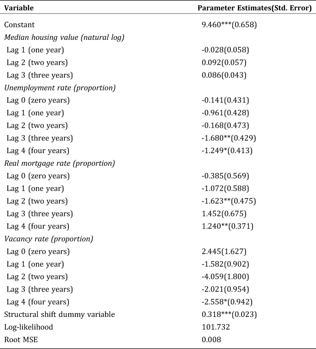
Table A3. Scenario-Specific and Expected Optimal Budget Allocations across the Five Clusters Corresponding to the Four Points on the Mean-Variance Trade-Off Frontier in Figure A1 as a Sensitivity Test using TN per capita GDP

Table A4. Scenario-Specific Benefits and Costs, and Expected Benefits, Costs and ROIs Associated with the Four Pareto-Optimal Points along the Mean-Variance Trade-Off Frontier in Figure A1 as a Sensitivity Test using TN per capita GDP


Figure A1. Trade-off relationship between the Pareto-optimal total expected benefit of carbon storage and its variance as a sensitivity test using TN per capita GDP


 Open access