


Introduction
The development of regional food hubsFootnote 1 within food supply chains is interesting to researchers and policy makers for several reasons, such as supporting rural communities and agribusiness, supplying alternative food markets, and enhancing food security and sustainability (Brown and Miller Reference Buccola and Conner2008, Tropp Reference Tropp2008, King et al. Reference Matson, Thayer and Shaw2010, Martinez et al. 2010, Boys and Hughes Reference Brown and Miller2013, O'Hara and Pirog Reference O'Hara and Pirog2013, Bonanno and Li Reference Brown, Goetz and Ahearn2015, Jablonski, Schmit and Kay Reference Jacobs2016). In the public realm, the US Department of Agriculture (USDA) promotes various policies and programs to strengthen local economies and food systems. The USDA's “Know Your Farmer, Know Your Food” initiative, for example, sought to better connect farmers and consumers while supporting local and regional food systems (Reference King, Hand, DiGiacomo, Clancy, Gómez, Hardesty, Lev and McLaughlinUSDA n.d.). The development of regional food hubs can be key to this strategy.
Hubs are a key component of food value chains (Hardesty et al. Reference Ippolito2014, Ge et al. Reference Ge, Goetz, Canning and Perez2015). Even as demand for local food has created new marketing opportunities for producers (Brown et al. Reference Boys and Hughes2014), it is difficult for smaller and mid-sized farms to access rapidly growing retail, institutional, and commercial foodservice markets. On the other hand, large buyers, including institutions, restaurants, and grocery stores, have difficulty finding local producers who can consistently supply food. In many cases, individual farmers are limited in their ability to satisfy a large buyer. By offering a suite of aggregation, distribution, and marketing services, food hubs enable farmers to gain entry into new large-volume outlets (Barham et al. Reference Bonanno and Li2012) while allowing larger buyers to meet the growing demand for local foods (Matson et al. Reference Novaco, Stokols and Milanesi2015). In this way, food hubs connect producers of all sizes into mainstream food procurement and distribution systems and facilitate large-scale buying of farm products with desired attributes at lower costs.
In this paper, we examine the hub location problem, focusing on the case of the US fresh produce supply chain.Footnote 2 Fresh produce has two important traits—perishability and seasonality. In this study, we segment the post-harvest fresh produce value chain into two stages: (i) aggregation of seasonal domestic harvest plus imports by domestic first-handlers, and (ii) marketing of all first-handler seasonal inventory to domestic and export buyers serving the consumer market. Our research focuses on the first-handler problem, and although, in practice, many first-handler establishments may also be growers, retailers, or exporters, they all confront the problem of procuring large volumes and varieties of highly perishable produce from individual farms as quickly and efficiently as possible. This segmentation of the first-handler stage for what is increasingly a vertically integrated value chain allows for subsequent modeling (beyond the scope of this research) of trade between first-handler regional hubs holding all seasonal inventories, called aggregation hubs in this study, and consumer marketing area buyers representing all regional markets.
Aggregation hub sizes and locations significantly impact the marketability of a region's fresh produce, as well as its viability as a site for fresh produce imports. This study will build an optimization model to identify the optimal locations and scale for county-level aggregation hubs sourcing from growers and importers located in multiple US counties. In doing so, we identify characteristics of a nationally coordinated optimal hub system, in part to examine if these characteristics are determinative of the structure of our current system. Our study attempts to answer some key questions for policymakers, investors, or hub operators around selecting hub locations, determining operating costs, and developing efficient strategies to operate hubs seasonally.
Hub location decisions are crucial determinants of supply chain efficiency for the aggregation and distribution of products. Here we characterize and model an optimal US network of fresh produce assembly in which hub sizes and locations at county-level are endogenously determined. The hub network minimizes total costs of assembling US domestically produced fresh produce products for domestic consumption plus imports from other regions beyond the US. This study falls within the scope of strategic planning for facility location of supply chains, where optimization models have proven useful for solving heuristic decision-making problems (Buccola and Conner Reference Camargo, Miranda and Luna1979, Alumur and Kara Reference Alumur and Kara2008, Ge et al. Reference Ge, Goetz, Canning and Perez2018a). However, previous comparable applications to food systems (Jacobs Reference Jacobsen1972, Faminow and Sarhan Reference Ge, Canning, Goetz and Perez.1983, Etemadnia et al. Reference Etemadnia, Goetz and Canning2013, Etemadnia et al. Reference Faminow and Sarhan2015) use overly simplistic assumptions about hub operating patterns. First, they assume homogeneous operation costs across hubs with varying handling capacities when in fact scale economies are common in fresh produce supply chain systems and shape the optimal network configuration. Empirical evidence shows that the system cost function responds to quantity handled at hubs and rewards high quantity with a lower marginal cost (Cook Reference Dimiero and Mayfield2011, Ge et al. Reference Ge, Goetz, Canning and Perez2015, Reference Hardesty, Gail and Visher2018b). The lack of scale effects in earlier models means solutions likely deviate from actual market outcomes. Second, earlier studies use annual production data and ignore the seasonality in production that not only affects hub operational strategies but also creates heterogeneous costs across marketing seasons. Our study relaxes these assumptions.
To assess the role of scale economies in determining the structure of fresh produce aggregation hubs in a nationally coordinated system, we first estimate their cost functions using county-level cost and sales data of fresh fruit and vegetable wholesale establishments. Subsequently, we design four scenarios with different levels of scale effects and solve for optimal locations and scales of hubs at county-level. These optimal solutions are then visualized and analyzed. We then discuss implications of our findings on empirical approaches to model hub operations in applied food systems analysis.
The Effect of Scale Economies
Economies of scale play a fundamental role in network design and operations decisions, and thus affects network performance (Camargo et al. Reference Canning2009). Hubs operating on a large scale enjoy lower operating costs compared with smaller-scale hubs (King Reference Martinez, Hand and Pra1973, Jacobsen Reference King2013). Large-scale operations experience more efficient aggregation, storage, distribution, and marketing of products from local producers to consumers (Matson et al. 2013). As a result, smaller hubs face challenges, such as inefficiency in operating those hub agribusiness services for local producers which allow for an increase in their operating costs and thus limit their ability to supply larger markets (Pressman and Lent 2013). If economies of scale are ignored in empirical estimates of the benefits from food system infrastructure investment and food system operations, the empirically generated optimal hub network solution could be misleading (Ippolito Reference Jablonski, Schmit and Kay1975).
In this study, the characteristics and functionalities of modeled aggregation hubs are more similar to those mainstream and conventional aggregation and distribution facilities such as merchant wholesalers. The operation pattern of those counterparts in reality provides valuable information to build a model that mirrors the actual system. To measure scale effects inherent in fresh produce aggregation hub operations, we first compiled 2012 Economic Census data on annual sales and operating costs of fresh fruit and vegetable wholesale establishments (U.S. Census Bureau 2012). In many states, a subset of the counties are not reported for reasons of disclosure, so in these cases, we compile multicounty data by taking the difference between statewide totals and published county totals.Footnote 3 The resulting dataset is comprised of 114 county observations and 38 multicounty observations for (i) total annual operating costs, and (ii) total annual product sales.
Our hypothesis is that for a county (s) with a specific annual capacity (c) (the quantity handled at a county in a given year), annual operating costs (TCs) include a fixed component $\lpar h_c^0 \rpar$ that is independent of product volume handled, and a variable component $\lpar h_c^1 \rpar$
 that varies with volume handled (Q s). We consider sizes of regional aggregation hub operations C = 1 to c, where 1 is the smallest and c is the largest. Then the relationship between annual operating costs and county throughput of fresh produce is:

From the 152 county-wide observations of annual operating costs and throughput or hub sales, we convert the latter from dollars to pounds by dividing by the national weighted average 2012 wholesale price of 44.01 cents per pound for all fresh produce marketed in the United States (USDA National Agricultural Statistics Service 2018).
To represent the actual cost of hub operations in the model, we measure the effect of economies of scale inherent in hub operations based on our observations. Due to the limited number of observations, we disaggregate them into four groupings. After conducting sensitivity analyses with numerous groupings of the 152 observations, we identified and defined the four hierarchy groupings that provide the best empirical fit for the regression. The aggregation allows for the appropriate scale level for each grouping, which is based on the range of handled product quantity for observations in each grouping,
C 1: 130,000 units and below (36 lowest counties or equivalents by total annual throughput)
C 2: 130,001–450,000 units (next 39 counties by total annual throughput)
C 3: 450,001–1,500,000 units (next 39 counties by total annual throughput)
C 4: 1,500,001 units and above (highest 38 counties by total annual throughput)
To assess whether the mean values for the dependent variable (operating costs) differ between any two of the four groupings, we conduct two-tail t-tests between every two groupings. The absolute value of t-statistic ranges from 6.37 to 11.21. There is a statistically significant difference in the means of operating costs between groupings. We reject the null hypothesis that any two of the four groupings are equal.
For each grouping, the relationship between total operating cost (TC) and sales volume (Q) is obtained using OLS and shown in Table 1. The cost estimations will be used later to build the base scenario of the model.
Table 1. Regression Results for Economies of Scale Effect Based on 2012 Economic Census Data

Note: A single asterisk indicates significance at a 5 percent level, and a double asterisk indicates significance at a 10 percent level. These are county-level, not establishment-level hubs.Footnote 4
Source: Compiled by Authors based on U.S. Census Bureau (2012)
The regression results demonstrate a noticeable scale effect in hub operations. While fixed costs (intercept) increase with hub size, the marginal costs decrease with hub size. Specifically, the larger the hub size, the lower the marginal cost per unit (one thousand pounds) handled. In this manner, handling costs of an aggregation hub are based on the amount of product flow carried by the hub and endogenously respond to flow by rewarding the shipper for greater volumes shipped. Under cost minimization principles, the numbers and scale of facilities to be established typically are endogenously determined.
Each of the four marginal cost parameter estimates exhibits a highly significant t-statistic. While the fixed cost parameters are consistent with expectations and contribute to the overall goodness of fit in all four hub size equation estimates, they are also statistically significant at certain levels. Building on these results, the cost estimates in Table 1 are incorporated into the hub location model to demonstrate how they affect spatial network structures.
Data
USDA's National Agricultural Statistics Service (NASS) reports state-level annual production statistics for 21 different fresh market vegetable crops across 37 states (USDA National Agricultural Statistics Service 2018). The 2012 statistics are allocated to counties in these states based on harvested acreage by county, using the 2012 Census of Agriculture for total fresh market vegetables (USDA National Agricultural Statistics Service 2018). For states that are not covered in the annual NASS reports but are covered in the Census, harvested acreage data from the Census are multiplied by yield per acre data in nearby states to impute production.
In the Census data, harvested acreage of some counties is suppressed in order to protect the confidentiality of individual responders. To overcome data suppressions in the Census data, a constrained maximum likelihood mathematical programming model is used. The model minimizes adjustments to the variance-weighted initial estimates of suppressed county harvested acreage statistics to align these estimates with the adding up requirements of the hierarchical data in the 2012 Census. This hierarchy includes requirements that the sum of harvested acreage across all commodities equals the published county-wide total harvested acreage across all covered crops, and that the sum of harvested acreage for specific crops across all counties in a State equals the published statewide total for each crop. By simultaneously solving a state/county model and a national/state model for the same commodities, the model produces maximum likelihood estimates of all suppressed county harvested acreage statistics using the method described in Canning (Reference Cook2011). The same approach was used for estimates of both fresh market fruit production and fresh market vegetable production in US counties. Combined production for the subset of these 55 crops produced in each county is converted to a common unit (one thousand pounds) and summed to a single production statistic per county. Production estimated from suppressed county harvested acreage only accounts for a very small proportion of annual domestic production (1 percent) so the estimation error should have very limited influence on the aggregation hub location solution.
County-to-county shipping distances are based on the Oak Ridge National Laboratory multimodal impedance network data product, and average shipping cost statistics are reported by USDA Agricultural Marketing Service (Reference MacDonald, Korb and Hoppe2010).
According to 2012 USDA National Agricultural Statistics Service data, 2,467 counties, or 75 percent of all counties in the contiguous US, grew vegetables or fruits. Annual production statistics are disaggregated into seasonal marketing segments to more accurately account for the highly variable geographic disposition of annual fresh produce production. This is achieved by identifying the beginning and ending dates for the marketing seasons of each fresh produce crop in each state (USDA National Agricultural Statistics Service 2006, 2007). Many states have multiple growing regions with different marketing seasons for the same crop, and in some cases, a single crop may have two marketing seasons. Annual production data by county is allocated to each day of the identified marketing season(s) according to a normal distribution under the assumption that 100 percent of available product is marketed within 4 standard deviations of the marketing season midpoint. This imputed daily marketing data is then aggregated into four marketing seasons: January to March; April to June; July to September; October to December.
Monthly 2012 fresh produce import data by county of unladingFootnote 5 are compiled from U.S. Census Bureau (2012) sources. 81 counties in 30 states import fresh produce. Statistics reported in metric tons are converted to 1,000-pound units and aggregated into the same four marketing seasons as domestic production.
Figure 1 shows continental US fresh produce production plus imports mapped across four seasons. Production and imports are unevenly distributed across seasons, and the main production/import areas are on the West Coast and Florida. Among them, California has the highest production and import levels, followed by Florida and Washington. The Northeast and Upper Midwest also have high production and import levels, while production and imports in some Rocky Mountain States and Plains States are low.

Figure 1. Distribution of fresh produce production in the U.S. across seasons. (a). Production in Season 1 (January–March). (b). Production in Season 2 (April–June). (c). Production in Season 3 (July–September). (d). Production in Season 4 (October–December).
Market Setting and Optimization Model
Produce assembly at aggregation hub s involves shipment from surrounding production and import regions (or nodes) via a domestic freight network that connects all nodes and aggregation hubs. Volpe, Roeger, and Leibtag (Reference Volpe, Roeger and Leibtag2013) show that domestic shipments for produce commodities are almost exclusively by truck. It is assumed in this study all shipments are transported to regional hubs by truck. Transportation costs between node-hub pairs are often defined to be proportional to the distance between them. However, transportation costs are also subject to constraints, such as road condition, speed reduced on evening commute, and traffic congestion which influences travel time and speed (Novaco et al. Reference Pressman and Lent1990). To model transportation costs between production nodes and aggregation hubs, each link in the network is assigned an impedance value other than actual mileage. Impedance represents a measure of the amount of resistance, or cost, required to traverse a path in a network or to move from one element in the network to another. High impedance values indicate more resistance to movement. For this study, we use a national average shipping rate per impedance mile (the average cost of transporting 1,000 pounds of products for one impedance mile). If the shipping rate per impedance mile is converted to the shipping rate per highway mile, the latter is higher in more congested areas, and vice versa. We use county-to-county highway impedance measures from version 3 of the national multimodal impedance network database developed by Oak Ridge National Laboratory (Reference Teo and Shu2011), which is based on population weighted centroids.
Establishment home regions (business addresses) of fresh produce first-handlersFootnote 6 are increasingly based in key production areas, but they source from shifting production regions that follow climate-determined seasonal patterns throughout the year (Cook Reference Dimiero and Mayfield2011). To stay profitable, an establishment seeking to source from outside its home region must assemble and handle the produce at least as efficiently as establishments based in the originating region. Our approach is to design a national “home field” hub system where aggregation hubs built to one of the four scales reported in Table 1 are located throughout select growing/import regions in order to minimize total assembly and first-handler costs across all seasons and growing/import regions.
Whether the same hub locations and sizes would result from a model that allows for individual establishments to operate several “virtual hubs” in multiple locations is beyond the scope of this study. Such a model would require operating cost and throughput data that distinguishes between “home field” and “virtual” hub operations to calibrate the cost functions. Such data was not available for this study. We recognize that both types of operations exist in practice.
Our approach is realistic provided the cost structure of operating either hub type for a given annual throughput is similar. We are not aware of data or compelling arguments that suggest, a priori, a systematic bias is introduced by our assumption of similar cost structures. This issue does merit further investigation in future research. A practical limitation of our approach is the disconnect between the model results which report the physical location (county), cost, and throughput of all aggregation hubs, and the published Economic Census data which reports total costs and throughput reported by all establishments with business mailing addresses in each county. It is important that we be mindful of this difference when comparing the model results with the published data.
While the classic facility location model considers only a trade-off between facility fixed cost and transportation cost, this hub network design problem considers trade-offs between facility fixed cost, transportation cost, and operation cost (Teo and Shu 2004). We formulate this national hub system optimization problem as a mixed integer linear programming (MILP hereafter) model with the objective of minimizing total costs associated with product assembly and aggregation hub setups and operations. The optimization problem requires a definition of restrictions to ensure that total production and imports by county and average per unit supplier and shipping costs meet observed statistics. The following notation is introduced for the model:
Sets:
I = {1,…,i} denotes marketing seasons in a year;
F = {1,…,f} denotes a set of production locations;
S = {1,…,s} denotes a set of aggregation hub candidate locations;
C = {1,…,c} denotes capacity level of aggregation hubs; each capacity level has an interval span;
Parameters:
$p_{i\comma f}^{}$
 denotes production plus imports at location f in marketing season i;
$d_{f\comma s}^{}$
denotes distance between node location f and aggregation hub location s (impedance miles);t denotes fixed transportation cost ($ per thousand-pound impedance mile);
$h_c^0 \;$
denotes fixed annual handling cost of a c level aggregation hub;$h_c^1 \;$
denotes marginal handling cost per unit of annual throughput of a c level aggregation hub;$V_c^1 \;$
denotes maximum annual throughput of a c level aggregation hub;$V_c^2 \;$
denotes minimum annual throughput of a c level aggregation hub;


Variables:
$x_{i\comma f\comma s}^{}$
denotes quantity shipped from node f to aggregation hub s in marketing season i;$Z_{c\comma s}^{}$
denotes an integer variable = 1 if location s has an aggregation hub with capacity c, and 0 otherwise;Q s denotes annually assembled throughput for aggregation hub s;


Functions:
TC denotes system-wide total assembly plus first-handler costs.
The objective function and system constraints of a model to solve this problem are given in equations 2–9.
Minimize:

Subject to:


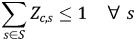


The objective function (Equation 2) minimizes the total cost, which includes fresh produce transportation (expression in second outer brackets) plus first-handler services (expression in first outer brackets). Equation 3 ensures that in each marketing season the total quantity transported from county f to all aggregation hubs S are equal to total quantity produced and imported in county f in the season. That is, all products must be assembled into aggregation hubs across marketing seasons. Equation 4 is an accounting identity, equation 5 provides the binary condition-build/not-build, and equation 6 ensures that 0 or 1 aggregation hub of scale c is built in county s. Equations 7 and 8 define the quantity-handling thresholds and limits for an aggregation hub of each capacity level. Together, equations 7 and 8 require that aggregation hubs of size c, for c = 1 to 4, will only be constructed in county s if it attracts enough shipments to meet its handling threshold $\lpar V_{c\comma s}^2 \rpar$ and does not attract shipments in excess of its handling limit $\lpar V_{c\comma s}^1 \rpar$
 . Equation 9 ensures that shipments only flow from nodes to aggregation hubs and not vice versa.
The model defined in equations 2–9 describes a national system of regional fresh produce aggregation hubs that seek to aggregate all available fresh produce sourced from US farms and US custom ports spanning vast geography. Any candidate hub location can offer lower per-unit operating costs as it reaches each of four handling thresholds with per-unit operating costs decreasing as each higher threshold is reached. But to reach each of the increasing threshold targets, a candidate hub location must aggregate produce from a larger geographic area. Achieving each higher level of aggregation will result in higher transportation costs. Candidate hub locations that can achieve these thresholds with lower transportation costs will be favored. For a solution to the model defined in equations 2–9 to be optimal, fresh produce originating across all locations cannot decrease its combined aggregation (transportation) and handling costs by redirecting any product to a different aggregation hub location in any marketing season.
Model Setting
In this study, the handling capacity of an aggregation hub is the quantity that can be managed at the aggregation hub during a given year. To incorporate scale effects inherent in aggregation hub operations into the model, we use the operating cost estimates reported in Table 1. The handling capacity of hubs defined for our regression analysis also defines the four different annual thresholds for the quantity of products handled at aggregation hubs over the four marketing seasons. Following the regression pattern of operating costs reported in Table 1, when the scale effect is present, an aggregation hub handling a higher quantity of products enjoys lower marginal costs. An aggregation hub must handle a minimal level of product quantity to achieve a certain level of scale effect, and this motivates the construction of large capacity aggregation hubs.
In reality, factors influencing hub operations and maintenance are complex. The food system has experienced significant changes over the past decades and today's food system has been shaped historically by a range of internal and external social and economic drivers that have evolved with time as well. In this study, the regression results for fixed costs and marginal costs quantitatively reflect the effects of different influential factors at an aggregation level. Fresh produce facility operating data from the 2012 Economic Census indicate the increased dominance of large-scale facilities in fresh produce assembly and distribution across the US when compared with data from the 2007 Economic Census. The marginal cost margin in regressions of 2012 data increases when compared with the regression results using 2007 annual sales and operating costs data (see Table A1 in Appendix I). Here the marginal cost margin is defined as the marginal cost difference between two adjacent aggregation hub levels. The difference between sets of results indicates a possible trend of a more pronounced scale effect stemming from scaling up hubs in the future. In order to identify the effect of scale economies on the optimal solutions of the problem, we design four scenarios in which different values of the marginal handling costs are assumed.
We set Scenario 1 as a scenario in which the marginal cost is not related to economies of scale. The cost remains constant across aggregation hub levels, that is, $55.74, which is the marginal cost of Level 1 aggregation shown in Table 1. Scenario 1 captures the incremental costs of building to a larger scale while omitting the incremental efficiencies realized by scaling up. We will demonstrate how the modeling results in Scenario 1 will differ from those of the base scenario (Scenario 2) as the existing scale effect is ignored.
Scenario 2 is designed as the base scenario in which the marginal costs to handle 1,000 pounds of product for four levels of aggregation hubs follow the regression results shown in Table 1, that is, $59.74, $49.71, $38.67 and $36.89 for aggregation hub Levels 1 to 4, respectively. The marginal cost margin between Level 1 and Level 2 aggregation hubs is $10.03. This value is $11.04 between Level 2 and Level 3 aggregation hubs, and is $1.78 between Level 3 and Level 4 aggregation hubs. Empirical estimation of operating costs based on more recent observations are more likely to appropriately reflect the current operational environment for hubs, so the solution of Scenario 2 can provide empirical implication for the optimal structure of a hub network in the current situation.
To allow for the possible trend of more pronounced scale effect in the future, two additional scenarios are designed. Based on the base scenario, we increase the marginal cost margins between aggregation hub sizes by 20 percent to generate new marginal costs for the four aggregation hub sizes in Scenario 3, and increase the margins by 40 percent for setting up Scenario 4. Eventually, the fixed and marginal costs for each aggregation hub size in each scenario are listed in Table 2. The magnitude of scale effect increases from Scenario 1 to Scenario 4.
Table 2. Fixed Costs and Marginal Costs for Hubs

a Note: C 1: 130,000 units and below; C 2: 130,001–450,000 units; C 3: 450,001–1,500,000 units; C 4: 1,500,001 units and above (unit: one thousand pounds).
b Note: Scenario 1- no scale effect on marginal cost; Scenario 2- base scenario; Scenario 3–20 percent increase in marginal cost margin; Scenario 4–40 percent increase in marginal cost margin.
Results and Analysis
A heuristic algorithm is designed to determine the optimal solutions of the model. The heuristic procedure is iterative, starting with an arbitrarily chosen set of random initial locations for given numbers of aggregation hubs with varying handling capacity levels, and then allocating production nodes to these aggregation hubs. The iterative procedure of the optimization model is repeated to gradually improve these locations and leads to the minimum total costs. The optimal-seeking procedure will be terminated as soon as an effective solution is obtained. The optimization problem is compiled using GAMS and solved using CPLEX. All computational executions were performed on a High-Performance Computing System.
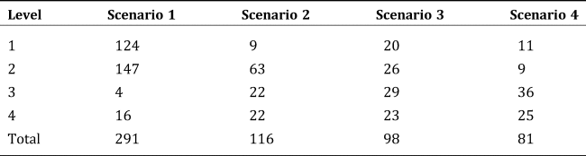
The aggregation hub numbers at each level across scenarios change significantly due to the scale effect. While the higher fixed cost of operating an aggregation hub with large capacity and shipping costs reduces incentives to build a large-capacity aggregation hub, the cost advantages of a large-capacity aggregation hub over a small-capacity aggregation hub provide incentives for sourcing products farther away in order to build a large aggregation hub. There is a trade-off between the increase in fixed costs and shipping costs to build a large aggregation hub and saved variable costs stemming from operating a large aggregation hub. If the latter outweighs the former, building a large aggregation hub at a hub location will be more profitable. The model is designed to determine the optimal balance between these cost components. As shown in Table 3, the numbers of smaller-scale aggregation hubs (Level 1 and 2) are negatively related to the marginal cost margin and, conversely, the numbers of larger scale aggregation hubs (Level 3 and 4) are positively related to the cost margin. Obviously, the presence of a more pronounced scale effect discourages small-scale aggregation hubs and encourages larger-scale aggregation hubs.2
Table 3. The Number of Aggregation Hubs at Each Level Across Scenarios
The locations and scales (annual handling capacity) of these aggregation hubs in each scenario are shown in Figure 2. For each scenario, counties served by aggregation hubs at different levels are marked in different colors on the map. The optimal solutions of Scenarios 1 to 4 are sensitive to the change in marginal handling costs for aggregation hub levels. If the marginal cost margin between levels changes, a new solution is required to meet a new optimum that takes advantage of the comparative costs. There are significant changes in aggregation hub location solutions in response to the change in the magnitude of scale effect. Also, product assembly patterns for aggregation hubs at each level differ significantly across scenarios.

Figure 2. Model Solutions. (a). Solution for Scenario 1. (b). Solution for Scenario 2. (c). Solution for Scenario 3. (d). Solution for Scenario 4.
The model captures production seasonality and thus introduces more flexibility in choosing the values of control variables involved in the model (i.e., the volume of seasonal product transported from production and import nodes to aggregation hubs) than a model ignoring production seasonality. To utilize the hub capacity efficiently and take advantage of scale effects, hub operators need to adjust assembly practices to match the production and import seasonality. The model displays the most efficient strategies for allocating production and imports in different counties into different aggregation hubs in different seasons. Consequently, solutions generated by the seasonal model are more consistent with actual aggregation hub practices and lead to 0.91 percent lower systematic costs than a model ignoring seasonality. Hence, the seasonal model solution is practical and effective for informing investment and policy decision makers regarding developing regional and local food systems.
As shown in Figure 2, while there is a divergence between aggregation hub locations in different scenarios, there are also some overlaps of optimal hub locations between scenarios. A possible explanation is that whenever operational conditions change, counties that enjoy high production plus import levels, or that can source products easily from surrounding counties, are ideal candidates for aggregation hubs. Table 4 shows the number of overlaps of aggregation hub locations between scenarios. Cells in the 4 × 4 matrix in Table 4 indicate the number of aggregation hub location overlaps between scenarios and the relative ratio of overlap. The main diagonal of the matrix shows the total number of aggregation hubs for each specific scenario.
Table 4. Comparative Hub Location Overlap Matrix

Even if these aggregation hubs use the same locations in different scenarios, as shown in Figure 2, the aggregation hubs may differ in scale and sourcing counties from where they assemble. The varying magnitudes of economies of scale provide varying levels of incentives to adjust the hub network structure for accommodating changes in operational conditions and achieving the minimum handling costs.
With the scale effect, aggregation hubs handling a larger quantity of products enjoy lower marginal handling costs. The merging of smaller aggregation hubs into larger aggregation hubs leads to handling cost savings. Hence, as the marginal cost margin between levels increases, the incentives to establish more aggregation hubs with larger capacity increase. To obtain the full benefit of economies of scale, the distribution of products among aggregation hubs becomes strategic in order to reduce handling costs. Just as Figure 3 shows, the total quantity handled in Level 2 aggregation hubs decreases with the magnitude of scale effect while the total quantity handled in Level 3–4 aggregation hubs increases with the magnitude of scale effect. We noticed that the change in quantity handled in Level 1 aggregation hubs remains ambiguous when the marginal cost margin increases. But our results show that the total quantity handled at Level 1 facilities in Scenario 2–4 is less than 2 percent, meaning that the Level 1 facilities play a minimal role in explaining the effect of scale of economics on the optimal solution of aggregation hub locations.
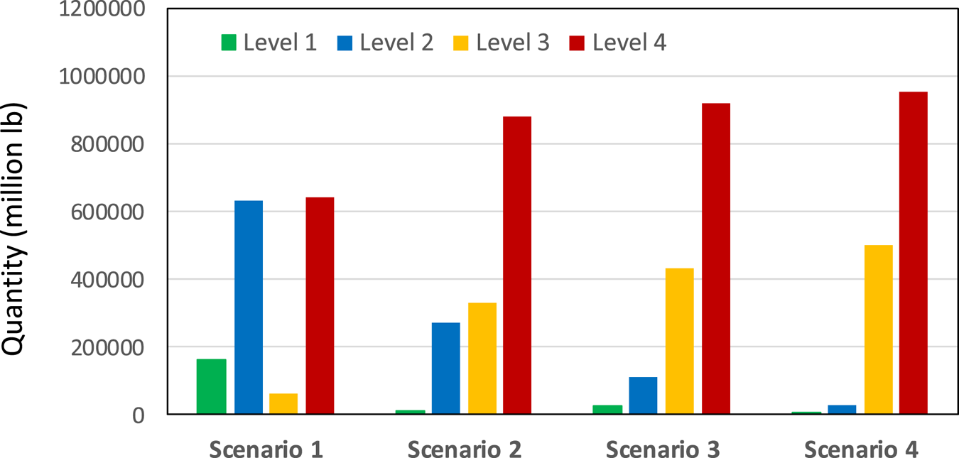
Figure 3. Total quantity handled at each level across scenarios.
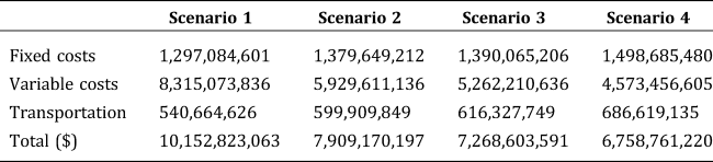
The marginal cost between aggregation hub levels provides incentives for transporting products longer distances in order to build upper-level aggregation hubs which take advantage of the scale effect. As shown in Table 5, transportation costs increase with the marginal cost margin between aggregation hub levels, implying that the accumulated total transport miles increase from Scenario 1 to Scenario 4. As a result, average transportation distance for one unit of product is 45, 50, 52, and 58 miles for Scenarios 1–4, respectively.
Table 5. Relative Costs Across Scenarios
Conclusion and Discussion
The presence of significant economies of scale in the fresh produce value chain complicates the aggregation hub location problem. Allowing for the effect of economies of scale inherent in hub operations for both present and future situations, this study designs several scenarios to assess the scale effect of economies on the solution of optimal aggregation hub locations. As expected, economies of scale play an essential role in shaping the food network structure. Our results provide strong evidence that scale effects have a significant impact on aggregation hub location solutions. Under different marginal cost assumptions, produce transportation is re-routed to take advantage of cost saving, and thus the structure of the network is reshaped. When the marginal handling cost margin increases, more aggregation hubs with large capacity emerge while the number of small capacity aggregation hubs diminishes. If economies of scale inherent in hub operations are ignored, the generated hub location solution could be misleading. Our modeling methodology and model solutions may provide valuable information to make improvements in the overall efficiency of the logistics of the networks as they adapt to possibly changed conditions of their economic environment. This study generates several products that will be of interest to researchers, industry practitioners, and government officials concerned with strategy and policy issues. Those issues include investing in regional food hub infrastructure, developing policies and programs promoting regional and local food systems, and increasing efficiency in hub operation to remain viable and competitive.
Larger farms are realizing better economic returns than smaller farms in the United States, where a doubling of farm size has occurred over the past 20 to 25 years (MacDonald et al. Reference Matson, Sullins and Cook2013). In this setting, we observe dominant US produce-growing regions serving consumer markets in lesser US produce-growing regions. Fresh produce first-handlers in key production areas are sourcing from other production regions (Cook Reference Dimiero and Mayfield2011), and our research establishes the presence and importance of scale economies in this intermediate industry. Our research indicates that distributional implications of this market setting are an outstanding empirical question. The modeling approach used in this study informs both analytical and empirical approaches to assessing the possible welfare and policy implications of the current spatial and vertical market structures among the broad spectrum of fresh produce that is grown, imported, exported, and marketed throughout the United States.
The model has several limitations that suggest topics for future investigation. Addressing the effects of scale economies by explicitly considering them as a cost in the objective function is a more realistic modeling approach. But specifying a suitable cost function that allows for scale effects is not a simple matter. Our efforts to assess the impact of economies of scale suffer from insufficient data necessary for a complete evaluation. In this study, the assumption of fixed and per unit marginal handling costs for each capacity choice are informed by regression analysis of data based on a limited number of observations and a rough, initial classification. To fully advance the modeling of these types of economic issues, more investigation is needed to better understand the pattern of scale effects and its influence on hub operation costs.
The model is based on an assumption that first-handlers seek to aggregate all seasonal produce as quickly and efficiently as possible in order to offer the best free-on-board price (price that excludes the cost of shipment to the buyer) to all potential buyers. An alternative model could also factor in the demand side by coordinating aggregation and distribution functions for locally or regionally sourced produce. Aggregated products in these aggregation hubs will be in greater proximity to distribution centers or points of retail purchase. But whether this consideration influences optimal aggregation locations is an empirical question. Just as production volumes by geographic location are uncertain due to factors such as weather, crop diseases, and pest infestations, the consumer markets served by each aggregation hub can be highly uncertain due to these same factors on a worldwide scale. Such uncertainty is also intensified by the increasing share of the consumer produce market being served by very large volume buyers representing large retail and foodservice chains. Existing data on fruit and vegetable wholesalers do not distinguish between first-handlers and establishments sourcing their produce from someone other than the growers, so empirical tests of demand side factors on optimal aggregation locations are difficult. Other perishable foods with more readily identifiable node-to-hub transactions, such as the numerous fresh meat value chains, may allow empirical hypothesis testing of these competing models.
Finally, in this study, the hub location problem involves a large-scale optimization model. The amount of memory and the computational effort needed to solve such problems grow significantly with the number of variables and constraints. To solve the model with a reasonable computation time, we avoid extensive identification of the varieties of fresh produce commodities at the county-level. Actually, a consumer's consumption of produce products differs across varieties. Once the influence of retail markets on hub locations is taken into consideration in a model, it is necessary that different hubs apply different assembly strategies regarding different varieties of imported or domestically grown produce. Further studies should allow for produce category differentials instead of assuming all products are homogenous. Overcoming these limitations can make the model generate more realistic solutions that capture actual assembly patterns of the system.
Acknowledgments
This research was supported in part by the US Department of Agriculture (USDA) under USDA NIFA grant no. 2011-68004-30057 and under a cooperative agreement with USDA ERS no. 58-4000-5-0017. The findings and conclusions in this publication are those of the authors and should not be construed to represent any official USDA or US Government determination or policy. The authors want to thank the Editor for the input into this article. Insightful comments from two anonymous referees were also very much appreciated.
Appendix I Scale Effect Regression Using 2007 Data Samples
We collected and compiled 2007 Economics Census data (U.S. Census Bureau 2010). From the 108 county-wide observations of annual operating costs and throughput or hub sales, we convert the latter from dollars to pounds by dividing by the national weighted average 2007 wholesale price of 31.3 cents per pound for all fresh produce marketed in the United States (USDA National Agricultural Statistics Service 2009a, 2009b, 2009c, 2009d).
The aggregation allows for the appropriate scale level for each grouping,
C = 1: 130,000 units and below (27 lowest counties or equivalents by total annual throughput)
C = 2: 130,001–450,000 units (next 34 counties by total annual throughput)
C = 3: 450,001–1,500,000 units (next 26 counties by total annual throughput)
C = 4: 1,500,001 units and above (highest 21 counties by total annual throughput)
Again, we conduct two-tail t-tests between each two of the two groupings. The absolute value of t-statistic ranges from 6.37 to 11.21. We reject the null hypothesis that any two of the four groupings are equal. For each grouping, the relationship between total operating cost (TC) and sales volume (Q) is obtained using OLS (Table A1).
Table A1. Regression Results for Scale Effect of Economies (Fresh Produce)


 Open access