


In 2010, the U.S. Environmental Protection Agency (EPA) established the Chesapeake Bay Total Maximum Daily Load (TMDL) under the Clean Water Act with the goal of reducing nitrogen by 25 percent, phosphorus by 24 percent, and sediment by 20 percent by 2025, with at least 60 percent completed by 2017 (U.S. Environmental Protection Agency 2010). Even though the Chesapeake Bay watershed spans 6 states (Delaware, Maryland, New York, Pennsylvania, Virginia, and West Virginia) and the District of Columbia, Pennsylvania provides 50 percent of the Bay's total freshwater flow and contributes 47 percent of the nitrogen load, 26 percent of the phosphorus load, and 32 percent of the sediment load (Environmental Finance Center University of Maryland 2016). Although the results of the Chesapeake Bay TMDL 2017 midpoint assessment are not available yet, it is clear that Pennsylvania did not meet its 2017 pollution milestones and needs to reduce nitrogen levels by 34 million pounds per year (a 43 percent reduction from 2016 levels), phosphorous levels by 0.7 million pounds per year (a 20 percent reduction), and sediment levels by 489 million pounds per year (a 25 percent reduction) by 2025 with the majority of these reductions coming from the agricultural sector – 27 million pounds per year of nitrogen reduction (80 percent of the total reduction), 0.685 million pounds per year of phosphorous reduction (98 percent), and 412 million pounds per year of sediment reduction (84 percent) (Chesapeake Bay Program 2017).
The cost of achieving these pollution reduction goals is unclear. The Chesapeake Bay Commission (2012) estimated that the median costs are below $100 per pound of nitrogen and below $1,000 per pound of phosphorus for agricultural best management practices (BMPs). Shortle et al. (Reference Shortle, Kaufman, Abler, Harper, Hamlett and Royer2013) estimated the value of reduced pollution under a nutrient credit trading scenario using price points ranging from $2 to $20 per pound of nitrogen and $10 to $100 per pound of phosphorous. Shortle et al. (Reference Shortle, Kaufman, Abler, Harper, Hamlett and Royer2013) also estimated that to implement all the agricultural BMPs in Pennsylvania's Watershed Implementation Plan (WIP) it would cost $378.3 million per year between 2011 and 2025. However, it is not guaranteed that these BMPs would achieve the required nutrient and sediment reductions. Using payments for agricultural practices that reduce nitrogen pollution in Maryland, Woodbury et al. (Reference Woodbury, Kemanian, Jacobson and Langholtz2017) estimate a price of $5.90 per pound of nitrogen reduction. Given that the agricultural sector in Pennsylvania must reduce nitrogen pollution by 27 million pounds per year by 2025, this yields an estimate of around $160 million per year to achieve Pennsylvania's nitrogen goals. Currently approximately $140 million of federal and state funding is spent per year on reducing Pennsylvania's nonpoint source pollution with 87 percent going toward BMPs (Environmental Finance Center University of Maryland 2016).
Given the funding gap between the amount currently spent on reducing nutrient and sediment pollution from agriculture in Pennsylvania and the amount needed to achieve Pennsylvania's TMDL, the EPA has recommended targeting funds for effective agricultural BMPs in high priority areas where nutrient reductions are the most effective (see Figure 1). This study compares the nitrogen reduction benefits from a targeted BMP strategy where payments for ecosystem services (PESs) are based on nitrogen reduction effectiveness with a uniform payment strategy where PESs are based solely on implementation of a BMP. Targeted PESs are most effective when the areas that are most effective at providing environmental benefits are also the areas that require the highest payments (Wunder Reference Wunder2007; Clements et al. Reference Clements, John, Nielsen, An, Tan and Milner-Gulland2010). However, targeted PESs have increasingly come under scrutiny as paying for services that would be provided in the absence of government intervention. This would be the case if the areas that provide the highest benefits are also the areas that are mostly likely to adopt BMPs. We explore the water quality benefits under a targeted versus uniform PES that pays farmers to convert their cropland to second-generation bioenergy crops (i.e., nonfood crops used to produce bioenergy) to contribute to the literature on the effectiveness of targeted PESs.
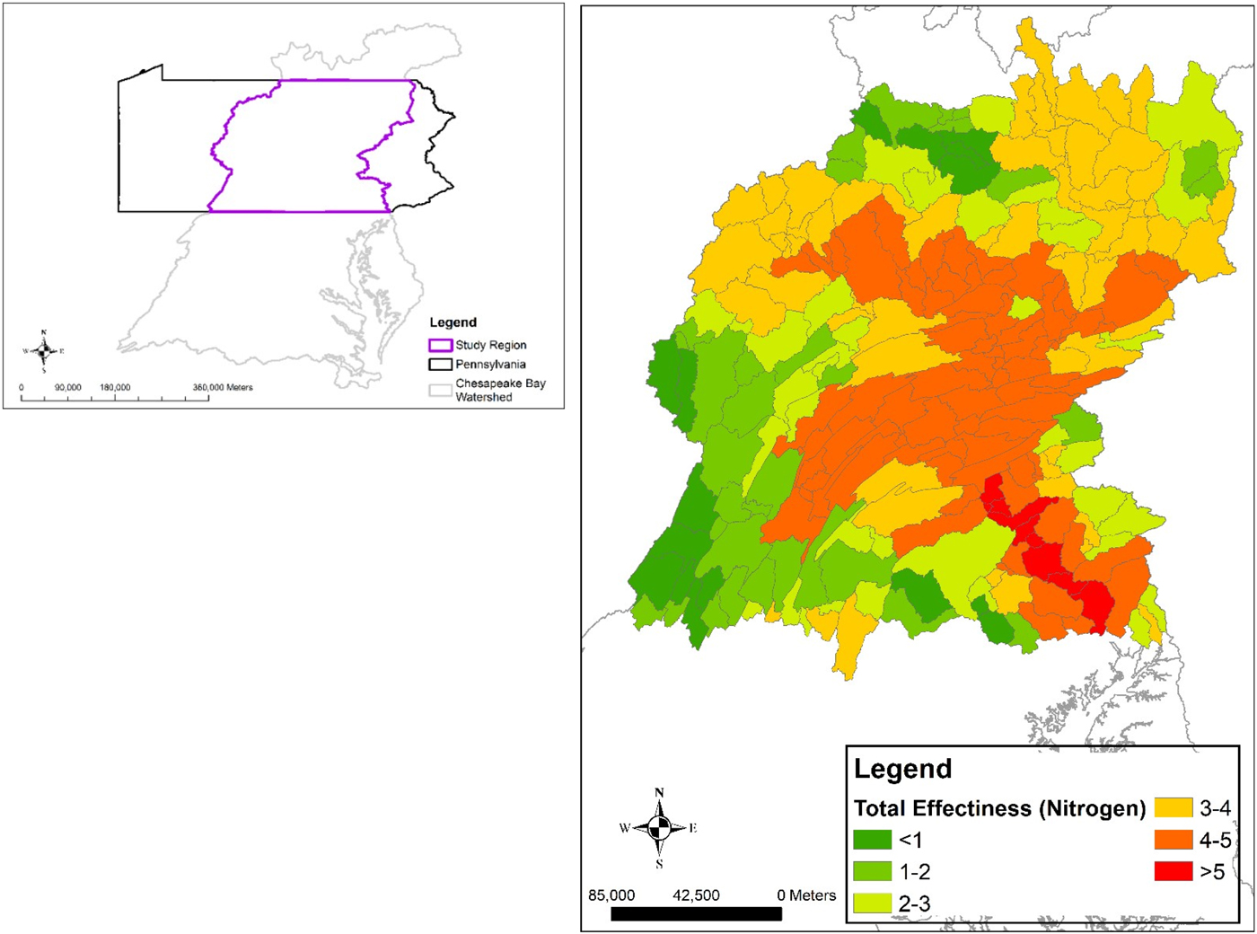
Figure 1. Relative Effect of a Pound of Nitrogen Pollution on the Chesapeake Bay Water Quality
In recent years, renewable energy fuels have gathered renewed interests as replacements for fossil fuels as a result of increasing concerns on various environmental issues (such as climate change and deforestation) and challenges to natural resources and ecosystems (such as watershed management and wetland conservation). Ethanol is the most common renewable fuel in the United States (English et al. Reference English, Ugarte, Walsh, Hellwinckel and Menard2006), and currently mainly comes from corn grain. However, corn ethanol has come under increasing scrutiny for its high dependence on nitrogen fertilizer and other fossil energy inputs (Camargo et al. Reference Camargo, Ryan and Richard2013), as well as impacts on food markets (Mueller et al. Reference Mueller, Anderson and Wallington2011; Zilberman et al. Reference Zilberman, Hochman, Rajagopal, Sexton and Timilsina2012). Hence, cellulosic ethanol, which is generated from inedible plant parts, has been recognized as a more attractive alternative to corn-ethanol. Compared with corn, these second-generation biofuel crops like switchgrass require fewer nutrient and chemical inputs such as nitrogen, phosphorus and pesticide while also having high potential for soil carbon sequestration and erosion prevention, and higher energy conversion efficiency in ethanol production (English et al. Reference English, Ugarte, Walsh, Hellwinckel and Menard2006; Ugarte et al. Reference Ugarte, English, Jensen, Hellwinckel, Menard and Wilson2006).
Yet second-generation biofuel production in the United States is not at a large enough scale to accomplish these environmental services or to meet federal mandates,Footnote 1 due to lack of land dedicated to bioenergy crops in current agricultural production (Thompson et al. Reference Thomson, Izarrualde, West, Parrish, Tyler and Williams2009). Furthermore, there is not sufficient idle cropland to grow the necessary biomass crops (Lubowski et al. Reference Lubowski, Vesterby, Bucholtz, Baez and Roberts2006). Hence, there is potential need for large scale land-use conversion from current crops like corn and soybeans toward cellulosic biofuel crops.
However, there are several factors that may hinder the necessary land-use conversions from current crops to biofuel crops such as switchgrass. First, switchgrass yields are often observed to be generally lower than expected potential yields, as switchgrass crops are vulnerable to impacts from spatial variation of soil features, landscape, precipitation, weed competition, pests, disease and temperature (Di Virgilio et al. Reference Di Virgilio, Monti and Venturi2007; Wullschleger et al. Reference Wullschleger, Davis, Borsuk, Gunderson and Lynd2010). Second, there exists volatility in the expected returns to switchgrass due to fluctuations in associations with gasoline pricesFootnote 2. Third, in the current market for switchgrass growers, the expected revenues from switchgrass are often offset by the relatively high maintenance, transportation and other costs (see, e.g., Qin et al. Reference Qin, Mohan, El-Halwagi, Cornforth and McCarl2006; Jin et al. Reference Jin, Larson and Celik2009) as well as low efficiency in fuel transformation rate relative to corn-ethanol (Havlík et al. Reference Havlík, Schneider, Schmid, Böttcher, Fritz, Skalský and Aoki2011) such that it is not at advantage in comparison with the net returns from corn crops (Babcock et al. Reference Babcock, Gassman, Jha and Kling2007).
Payments for ecosystem services (PESs) offered by governments to farmers could be a solution to mitigate some of the uncertainties that lead to difficulties in switchgrass production and land use. Perennial grasses and winter energy crops, compared with conventional corn-soybeans crops, require much less nutrient and chemical inputs. In addition, these crops provide water quality improvements (Woodbury et al. Reference Woodbury, Howarth and Steinhart2008), carbon sequestration (Lee et al. Reference Lee, Owens and Doolittle2007), and prevent soil erosion (Kort et al. Reference Kort, Collins and Ditsch1998).
In particular, can PES for surface water quality improvements in the Chesapeake Bay Watershed in Pennsylvania from land conversion from corn-soybeans rotations to switchgrass be used to stimulate both bioenergy production and the necessary nutrient and sediment reduction required under the Chesapeake Bay TMDL? When private actions (e.g., growing perennial grasses) provide public goods for society (e.g., water quality benefits), there is an underprovision of the public goods. One way to ensure the optimal provision of public goods (e.g., water quality benefits from perennial crops) is for the government to offer a PES equal to the marginal benefit of the public good. For example, in European countries, the government subsidizes perennial energy crops as an important policy tool toward realizations of the European Union 2009/28 renewable energy target (e.g., Bocqueho and Jacquet Reference Bocqueho and Jacquet2010; Clancy et al. Reference Clancy, Breen, Thorne and Wallace2012; Krasuska and Rosenqvist Reference Krasuska and Rosenqvist2012). In the U.S., biofuel farmers who participate in the Biomass Crop Assistance Program (BCAP) can receive a matching payment up to $45 per dry U.S. ton (USDA 2011) for the establishment of eligible biomass crops to help achieve the mandates under the Renewable Fuel Standard.
Yet the question remains as how regulators can efficiently quantify the environmental benefits and ecosystem services that can be generated from the conversion of land use to perennial grasses. Indeed, although a uniform payment based on the aggregated observation of such benefits might often be seen in practice such as the annual PES paid to biofuel crop farmers by the USDA, it is likely unclear if it is the most effective policy tool due to variations and heterogeneity in the environmental performances as well as the costs for land use conversion, crop maintenance and productions that are not uniform. Hence targeted PESs have been increasingly championed as more efficient than uniform payments (Clements et al. Reference Clements, John, Nielsen, An, Tan and Milner-Gulland2010) if accurate estimates of the actual water quality benefits from land-use conversion are available to the regulators, and payments can be designed to accommodate these variations and set to be equal to the value of the nutrient reduction benefits. However, the benefits of targeted PES compared with uniform PES hinges on the correlation between environmental benefits provided and the cost of implementing BMPs. If areas that provide more environmental benefits are also the areas where the cost of implementing BMPs is the cheapest then uniform payments will not differ significantly from targeted payments. If, on the other hand, areas that provide more environmental benefits are the areas where the cost of implementing BMPs is the most expensive then targeted payments will be able to provide more cost effective environmental benefits.
In this study, we use a dynamic land-conversion model to predict farmer's decision to convert from a corn-soybeans rotation to switchgrass production in Pennsylvania under three scenarios: no PES, uniform PES (i.e., payment per acre planted in switchgrass), and targeted PES (i.e., payment per pound of nitrogen reduction in the Chesapeake Bay).
Our methodology follows Song et al. (Reference Song, Zhao and Swinton2011) but we make two contributions to answer a different research question: what are the water quality benefits of converting crop land from corn-soybeans to switchgrass under three scenarios – no PES, uniform PES (i.e., payment per acre planted in switchgrass), and targeted PES (i.e., payment per pound of nitrogen reduction in the Chesapeake Bay)? First, we include spatially heterogeneous corn-soybeans yields and switchgrass yields by dividing Pennsylvania into six segments according to the predicted benefit of nitrogen reduction to the Chesapeake Bay (see Figure 1). Yearly net returns for both crops are predicted to find the conversion boundaries from corn-soybeans to switchgrass and vice versa. Second, we add to the analysis a government PES for environmental performances. Hence, the effects of both the net return tradeoffs between switchgrass and corn-soybeans and the PES toward switchgrass are evaluated. For comparisons, we use both a uniform PES policy based on acres of switchgrass grown regardless of the water quality benefits generated and a targeted PES policy based on the predicted nitrogen benefits of switchgrass grown in different areas of Pennsylvania regarding the total effectiveness of the crop land in our simulations. Results suggest that the targeted PES policy is more effective than the uniform PES policy in stimulating the provision of nitrogen reductions, particularly in the long run. Furthermore, the cost per pound of nitrogen under a targeted PES policy is 8–19% lower than under the uniform PES policy.
Methodology
Dynamic Land-Use Conversion Model
We extend the dynamic land-use conversion model in Song et al. (Reference Song, Zhao and Swinton2011) to incorporate spatially varying economic performance and environmental benefits. Specifically, we expand the model by considering that the potential payoff for farmers who choose to convert from conventional crops to biofuel crops consists of not only the monetary values of crop yields, but also a one-time payment to offset conversion costs and an annual payment for ecosystem services (PES). The one-time payment (denoted as T cs) includes monetary compensation as well as technological assistance from government agencies to offset any fixed costs that farmers might incur if they accept the contract and convert their cropland from a corn-soybeans rotation (denoted as c) to biofuel crops such as switchgrass (denoted as s). In the United States, biofuel farmers who participate in the Biomass Crop Assistance Program can receive a one-time matching payment up to $45 per dry U.S. ton for two years (USDA 2011). For simplicity, consider that {c, s} is the only set of crop choices for a risk-neutral farmer with a unit of cropland, and any land-use conversion from i to j would incur a lump-sum cost C ij, i, j ∈ {c, s}.
The farmers' payoff consists of two components. First, the monetary value of yields from crop i in period t in area k is denoted by πik(t) which follows a stochastic process with evolution of a general form (Song et al. Reference Song, Zhao and Swinton2011), as follows:
 $$d\pi _{ik}\lpar t\rpar = \theta _{ik}\lpar \pi _{ik}\comma \; t\rpar dt + \sigma _{ik}\lpar \pi _{ik}\comma \; t\rpar d\varepsilon _{ik}\comma \; \quad i\in \lcub c\comma \; s\rcub $$
where the drift term θ ik(π ik, t) and variance σ ik(π ik, t) are observable nonrandom functions, and dε ik is the increment of a Wiener processFootnote 3 which allows farmers to learn about and predict future returns in each new period based on information updated in previous period. The correlation coefficient between the returns to c and s is denoted as ρ k, such that E[dε ckdε sk] = ρ kdt.
Second, farmers who convert their land use from corn-soybeans c, to switchgrass s can receive a PES from government agencies based on either the amount of area converted to switchgrass (uniform payment) or the generated environmental values (targeted payment) at the end of the period. Switchgrass and many other biofuels have the potential to provide a variety of environmental benefits such as soil nitrogen sequestration, water nutrient reduction, and biodiversity conservation (Hill et al. Reference Hill, Nelson, Tilman, Polasky and Tiffany2006). These benefits, although often not traded with market values, can be used by government agencies and regulators as a part of the efforts on environmental protection and ecosystem restoration. For simplicity, we denote the PES paid to farmers in each possible land use scenario in period t and area k as mφi(e kt), where φi(e kt), i ∈ {c, s} represents the environmental performance level of land use alternative i (e.g., pounds of nitrogen reduction per acre of switchgrass planted) perceived by government agencies at the end of period t in area k, and m is the PES rate (e.g., dollars per pound of nitrogen reduction). In an ideal scenario, the government's objective is to set the PES equal to the marginal damage from agricultural emissions (targeted payments). In the case of uniform payments, all farmers are offered the same PES regardless of the environmental performance (e.g., dollars per acre of switchgrass planted). Also, for conversion made from corn-soybeans to switchgrass, we assume that a one-time transfer T cs equal to the payment available from the USDA's BCAP program.
Farmers' expected present value payoff from crop returns on land use i at period t in area k is denoted V i(π ck(t), π sk(t)), which depends on the distribution of future returns of both land uses. Farmers make decisions between keeping their fields in land use i or converting it into alternative j, as:
 $$V^i\lpar \pi _{ck}\lpar t\rpar \comma \; \, \pi _{sk}\lpar t\rpar \rpar = max\left\{{\matrix{ {\pi_{ik}\lpar t\rpar dt + e^{-rdt}EV^i\lsqb {\pi_{ck}\lpar t + dt\rpar \times \pi_{sk}\lpar t + dt\rpar } \rsqb \comma \; } \cr {V^j\lpar \pi_{ck}\lpar t\rpar \comma \; \pi_{sk}\lpar t\rpar \rpar -C_{ij} + \gamma_{tk}^{cs}} \cr}} \right\}$$
which states that the optimal decision for farmers is made based on the comparison between the expected return from keeping the same land use i in the next period (the first term), and the expected return from converting to alternative j less the conversion cost C ij (the second term). If the land use conversion is made from c to s, the second term becomes  $ V^s\lpar \pi _{ck}\lpar t\rpar \comma \; \pi _{sk}\lpar t\rpar \rpar -C_{cs} + \gamma _{tk}^{cs} $, where $ \gamma _{tk}^{cs} \; = T_{cs} + m\phi _i\lpar e_{tk}\rpar $ represents the PES and the lump-sum payments from the government. The optimal decision is made by comparing returns of the status quo strategy (the first term) which involves returns from the land use type i and the option value of converting in the future with returns of the conversion strategy (the second term) which involves returns from the alternative land use type j and the PES payments less of the conversion costs and the option of converting back to the current land use in the future.
Conditions for Optimization
Hence, the optimal land use decision problem in equation (2), for value functions V i and V j, i, j ∈ {c, s}, must satisfy the following conditionsFootnote 4:
 $$ LV^i(\pi _{ck}({\rm t}),\pi _{sk}({\rm t})) \ge 0,i,j\in \{ c,s\} $$
where LV i(π ck(t), π sk(t)) is the second order Taylor expansion of V i(π ck(t), π sk(t)) by applying Ito's lemma, as:
 $$\eqalign{& LV^i\lpar \pi _{ck}\lpar {\rm t}\rpar \comma \; \pi _{sk}\lpar {\rm t}\rpar \rpar = {\rm r}V^i\lpar \pi _{ck}\comma \; \pi _{sk}\rpar -\pi _{ik}\lpar {\rm t}\rpar -\Sigma _{\,p = c\comma s}\alpha _p\lpar \pi _{\,pk\comma }{\rm t}\rpar \displaystyle{{\partial V^i} \over {\partial \pi _{\,pk}}}- \cr & \Sigma _{\,p = c\comma s}\displaystyle{{\sigma _p^2 \lpar \pi _{\,pk\comma }{\rm t}\rpar } \over 2}\displaystyle{{\partial ^2V^i} \over {\partial \pi _{\,pk}\partial \pi _{\,pk}}}-{\rm \rho} _k\sigma _c\lpar \pi _{ck}\comma \; {\rm t}\rpar \sigma _s\lpar \pi _{sk\comma }{\rm t}\rpar \displaystyle{{\partial ^2V^i} \over {\partial \pi _{ck}\partial \pi _{sk}}}} $$
 $$V^i\lpar \pi _{ck}\comma \; \pi _{sk}\rpar \ge V^j\lpar \pi _{ck}\comma \; \pi _{sk}\rpar -C_{ij\comma }i\comma \; j\in \lcub c\comma \; s\rcub \;and\, i\ne j$$
 $$\hbox{Either (3) or (4) holds with strict equality}.$$
Estimation and Data
The empirical method involves two steps. First, the return equation (1) is solved to find the analytical solutions of the parameters. Second, these parameters are calibrated in the value function equation (2) to estimate the optimal switching boundaries. The optimal switching boundaries determine both (i) the returns from switchgrass necessary to induce conversion from corn-soybeans to switchgrass given the returns the farmer can earn from corn-soybeans and (ii) the returns from corn-soybeans necessary to induce conversion from switchgrass to corn-soybeans given the returns the farmer can earn from corn- soybeans.
Parameter Estimation
First, returns from land use are assumed to follow stochastic processes, with unknown parameters including the drift term θ, variance σ ik and correlation between the two alternatives ρ k, which can be re-parameterized by linearization approximation. Two stochastic processes, geometric Brownian motion (GBM) and mean reversion (MR), are often used. Song et al. (Reference Song, Zhao and Swinton2011) used both dynamic processes to motivate their simulations, and stating that of the two random processes, GBM is often more widely used as a result of its analytical tractability. Hence in this study we use the GBM dynamic equations to estimate the necessary return parameters.
If the return equation follows GBM, the analytical representation is as follows:
 $$d\pi _{ik} = \theta _{ik}\pi _{ik}dt + \sigma _{ik}\pi _{ik}d\varepsilon _{ik}\comma \; \quad i\in \lcub c\comma \; s\rcub $$
Discrete approximation of the inter-temporal return difference gives:
 $$\ln \pi _{itk}-\ln \pi _{i\lpar t-1\rpar k} = \alpha _{ik} + \sigma _{ik}\varepsilon _{ik}\comma \; \quad i\in \lcub c\comma \; s\rcub $$
where we denote  $ \alpha _{ik} = \theta _i-{{{\sigma _{ik}{}^2}} \over 2} $, and errors εik follows standard normal distribution. The parameters α ik, σ ik and ρ k can be estimated by maximum likelihood method. Denote the sample mean of the series ln πitk − ln πi (t−1)k as μik and sample standard error as sik, then the maximum likelihood estimators for α ik and σ ik are $ \hat{\alpha} _{ik} = \mu _{ik} + {{{s_{ik}}{}^2} \over 2}\, {\rm and}\, \hat{\sigma} _{ik} = s_{ik} $. The estimator for the correlation coefficient ρ k is the correlation between the series of two land use types ln π ctk − ln π c(t−1)k and ln π stk − ln π s(t−1)k (Song et al. Reference Song, Zhao and Swinton2011).
Optimal Switching Boundaries
Second, the model is parameterized and solved by collocation using OSSOLVER (Fackler Reference Fackler2004) and estimated with CompEcon package in Matlab (MATLAB 2015; Miranda and Fackler Reference Miranda and Fackler2004). The value functions are approximated using a linearized combination of a sequence of known basis functions, such as:
 $$ {\widetilde{V}^i}\lpar \pi _{ck\comma }\pi _{sk}\rpar = \Sigma _{\,j_c = 1}^{n_c} \Sigma _{\,j_s = 1}^{n_s} c_{\,j_{ck}j_{sk}}\psi _{\,j_cj_s}\lpar \pi _{ck}\comma \; \pi _{sk}\rpar $$
where  $ c_{j_{ck}j_{sk}} $ is obtained when the decision optimality conditions are satisfied. The optimal decision rule is determined by solving and evaluating the approximated value functions at {c, s} as well as the return less the conversion costs, and based on the results the conversion strategy payoffs are then compared with the status-quo strategy payoffs (Fackler Reference Fackler2004).
A piecewise linear spline function is used as the family basis function, with the nodal points as the corresponding pairs of simulated returns for each state variable (net present value of return for each land use type) evenly spaced over the revenue interval between $0 and $1000, with an increment of $10. We solve for three scenarios – (1) no PES for the water quality benefits provided by switchgrass, (2) uniform PES of $100 per acre to farmers who convert current corn-soybeans land to switchgrass, and (3) targeted PES of $5.90 per pound of nitrogen reduction in the Chesapeake Bay. Our hypothesis ex ante is that, to the extent that the PES also lowers the variance in future switchgrass returns, PESs will reduce the boundary condition by more than the payment. For example, a PES of $100/acre could lower the returns from switchgrass required for farmers to convert their land by more than $100/acre if the PES significantly lowers the uncertainty of future returns. However, these payments also increase the value of the option value, which would incentivize farmers to keep their land in corn-soybeans and save the option to convert to switchgrass when prices are higher.
Simulated Land-Use Conversion
With the optimal switching boundary simulation results, it is possible to generate predictions on the expected probabilities that a given parcel of agricultural crop land will convert from corn-soybeans to switchgrass in a given year and vice versa. The procedure proceeds as follows (Song et al. Reference Song, Zhao and Swinton2011). Starting with the base year returns as the initial period (year zero) returns, use the estimated parameters from the GBM process in equation (7) to generate N = 5,000 Monte Carlo randomly drawn sample paths of joint returns for corn-soybeans and switchgrass for a 30-year time horizon: {π ck(t), π sk(t)}, t = 1, … 30. Following the same decision rule of optimal land-use conversion, in each period the returns for each sample path are compared with the corresponding conversion boundaries  $ \lcub b_k^{cs} \lpar \pi _{ck}\lpar t\rpar \rpar \comma \; b_k^{sc} \lpar \pi _{sk}\lpar t\rpar \rpar \rcub $ and it is determines if the current land use should be converted to the alternative land use or remain unchanged. For instance, for a parcel of corn-soybeans land, if in period t we find that $ b_k^{cs} \lpar \pi _{ck}\lpar t\rpar \rpar \gt \pi _{sk}\lpar t\rpar $ and the expected net return from switchgrass does not attain the required amount for conversion, then the land is kept in corn-soybeans. On the other hand, if $ b_k^{cs} \lpar \pi _{ck}\lpar t\rpar \rpar \le \pi _{sk}\lpar t\rpar $, meaning the expected net return from switchgrass is within the “conversion zone”, then the land would be converted from corn-soybeans to switchgrass. In the following period, the comparison is made against the b ksc(·) boundary to determine whether or not this parcel of land should be converted back to corn-soybeans or remain in switchgrass. The comparisons are iterated for each sample path over the 30-year period, then for each period the number of parcels of land being converted to switchgrass is counted (M). The predicted proportion of land being converted from corn-soybeans to switchgrass in each period is then obtained from dividing M by N.
Data
To explore the effects of PES on land-use conversion toward biofuel crops incorporating the heterogeneity in land characteristics, we divide the Chesapeake Bay watershed in Pennsylvania into river segments (see Chesapeake Community Modeling Program, n.d.) characterized by the respective relative effectiveness in nitrogen sequestrationFootnote 5. The land parcels are categorized into six sub-groupsFootnote 6 (average effectiveness for nitrogen reduction in parenthesesFootnote 7): total effectiveness (TE) below 1 (2.4 pounds/acre), between 1 and 2 (7.19 pounds/acre), between 2 and 3 (11.98 pounds/acre), between 3 and 4 (16.77 pounds/acre), between 4 and 5 (21.56 pounds/acre), and above 5 (26.35 pounds/acre) (U.S. Environmental Protection Agency 2010) (see Figure 1).
The total acreage of corn land of each group is calculated as weighted sum of the land parcels in the group by their fractions in each county. Similarly, we calculated the weighted sum of annual average yields and net returns from corn and switchgrass. We use the USDA data of acreage of land used for corn production at the county level and annual average corn yields in each county from 1996–2012 in Pennsylvania (USDA 2017), and used the simulated annual average yields of switchgrass in each county in Pennsylvania from (Daly et al. Reference Daly, Halbleib, Hannaway and Eaton2017). Then, we calculated the return per acre from corn-soybeans and switchgrass as the revenue from crop yields less operating costs incurred. In particular, because switchgrass is not a widely commercialized commodity, its price is not commonly observed. Song et al. (Reference Song, Zhao and Swinton2011) suggested that market price for ethanol can be used to approximate the price for switchgrass yield, and the farm-gate price of switchgrass received by farmers is calculated as the sum of market price for ethanol and government PES net of production and maintenance costs, conversion and transportation costs. First, the mean of switchgrass yield per acre is calculated from the simulation data to be 3.88 tons per acre. Second, we consider the production, maintenance and harvest of switchgrass. We assumed that the maintenance costs are $192 per acre (Penn State Extension 2014). Switchgrass farmers can receive an annual matching payment of up to $45 per dry ton if the feedstock is used for bioenergy (USDA 2011). Babcock et al. (Reference Babcock, Gassman, Jha and Kling2007) assume transportation costs to be $8 per ton. Third, switchgrass yields are converted to ethanol. The yield rate is assumed to be 79 gallons per ton of dried switchgrass (Penn State Extension 2014). Historical data for market price of ethanol are obtained from the market price data in Nebraska (Nebraska Energy Office 2016) following (Song et al. Reference Song, Zhao and Swinton2011). Because there is currently not a widely applicable commercial market for switchgrass crops in the U.S., ethanol prices are used to calculate the approximated revenues from switchgrass. The potential market demand for switchgrass in the region includes hay production, mushroom compost, poultry bedding, pellet mills (Ernst Conservation Seeds), biomass power plants (ReEnergy and Evergreen Power), and jet fuel (Renmatix, global headquarters in King of Prussia, PA, partnering with Amyris Biotechnologies). Future work can consider the impact of different potential markets on the supply of switchgrass, however, for the current analysis we only model switchgrass as an input for ethanol to be consistent with previous literature (Song et al. Reference Song, Zhao and Swinton2011). Table 1 summarizes all parameters used and sources of citations. With these parameters and the yield data, we calculate the weighted average net returns of corn and switchgrass for each group. A summary of the data by groups are presented in Table 2. Overall in the studied region, the average net real annual returns per acre are $168 for corn-soybeans, and $186 for switchgrass.Footnote 8 Two series of weighted average returns in the studied region are presented in Figure 2.
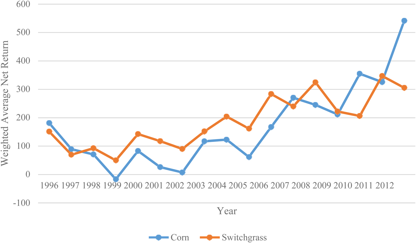
Figure 2. Weighted Average Net Return to Corn-Soybeans and Switchgrass in the Studied Region of Pennsylvania (1996–2012, in 2016 dollars)
Table 1. Parameters Used in Calculating the Net Returns of Corn-Soybeans and Switchgrass

Table 2. Crop Returns and Total Corn-Soybeans Acreage by Nitrogen Reduction Effectiveness: 1996–2012

Standard deviations in parentheses.
The targeted PES policy pays farmers who convert corn land to switchgrass in each group according to the group average effectiveness and a payment of $5.90 per pound of nitrogen reduced. The targeted PES paid to each effectiveness group range from $14.37 per acre for the lowest effectiveness group to $158.08 per acre for the highest effectiveness group.
For the uniform PES policy, we designate a hypothetical PES of $100 per acre for farmers with land used in switchgrass production, which corresponds to similar payments or budgets for cover crops in published policies, such as the $97 per acre annual budget for cover crops in Delaware's Chesapeake Watershed Implementation Plan (Delaware DNREC Reference Kauffman, Homsey, McVey, Mack and Chatterson2011) and $89 per acre annual payment for cover crops in Virginia's Agricultural BMP Tributary Action Strategy (Rephann Reference Rephann2010).
Using the annual return data and land use conversion costs, we estimated baseline parameters  $ \lcub \hat{\alpha} _{ck}\comma \; \hat{\sigma} _{ck}\comma \; \hat{\alpha} _{sk}\comma \; \hat{\sigma} _{sk}\comma \; {\widehat{{\rho_k}}}\rcub $ for each of the six nitrogen effectiveness sub-groups k using maximum likelihood estimators under three scenarios – no PES, uniform PES ($100/acre of switchgrass grown), and targeted PES ($5.90/pound of nitrogen reduced) are estimated. The estimated parameters for the six nitrogen effectiveness groups are presented in Table 3. These parameters determine the annual net return from either of the two land use types. Of particular interest in Table 3 is that the major effect of the uniform and targeted payments is on the variance of the switchgrass return, with the PES significantly lowering the variance of switchgrass returns. The conversion boundaries can be solved using the base year inputs and identify the optimal point for crop lands currently used for corn-soybeans production to be converted for switchgrass production, or vice versa.
Table 3. PES, Total Effectiveness and GBM Parameter Estimates by TE Group
Optimal Switching Boundaries
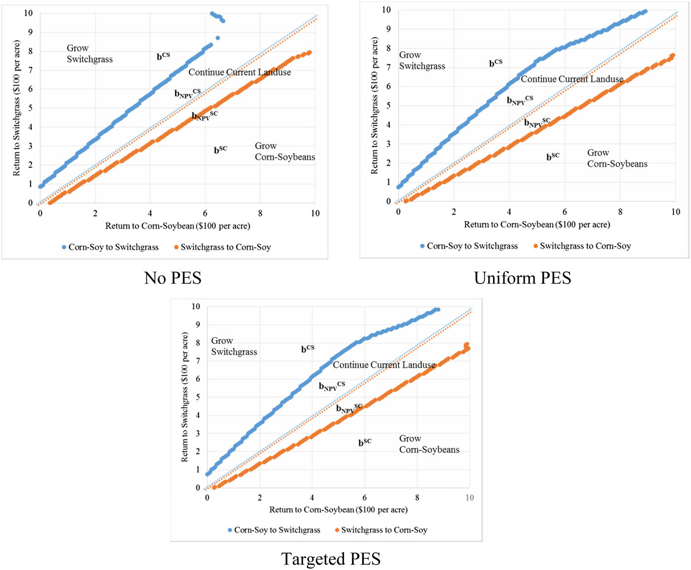
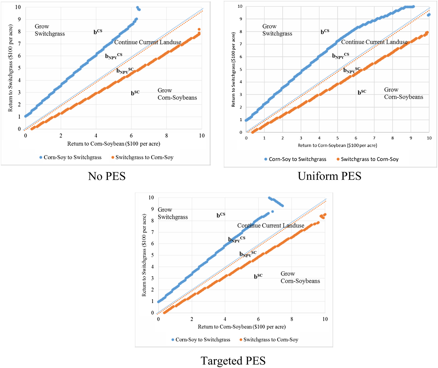
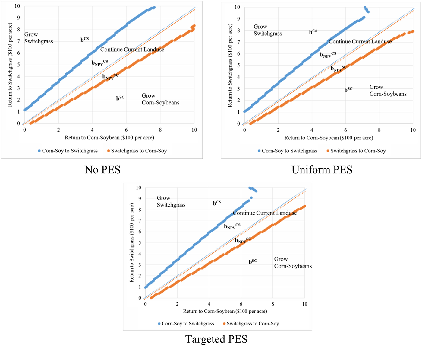
Optimal switching boundaries for the six groups with the three PES policies (No PES, uniform PES, and targeted PES) are obtained using OSSOLVER. These boundaries suggest necessary returns for farmers to make the land use conversion decisions from corn-soybeans to switchgrass, or vice versa. A summary of the optimal switching boundaries are presented in Table 4 and a full set of the graphs in the Appendix. For example, for the TE 0–1 group the weighted average net returns in 2009 is $121 per acre for corn-soybeans, and $198 per acre for switchgrass. The optimal switching boundary for conversion from corn to switchgrass is b(·), and the optimal switching boundary for conversion from switchgrass to corn is b sc(·). The two 45° lines represent the net returns if keep current land use unchanged. Hence, if the current land use is for corn production, the necessary net return to farmers to convert land use to switchgrass production is b cs(121) = $255 per acre in the no PES policy scenario, b cs(121) = $245 per acre in the uniform PES scenario, and b cs(121) = $245 per acre in the targeted PES scenario. In the no PES policy scenario the net return from switchgrass is $198 per acre, and in the targeted PES policy scenario the net return from switchgrass plus the targeted PES of $14.37 per acre is $213 per acre, both of which are less than the necessary return of $255 per acre, hence farmers would not incur conversion in these two policy scenarios. Meanwhile, in the uniform PES policy scenario the net return from switchgrass plus the $100 per acre PES is $298 per acre and higher than the necessary return, and the farmers would incur conversion.
Table 4. Dynamically Optimal Conversion Boundaries at Average Corn-Soybeans Returns (per Acre) and Average Switchgrass Returns (per Acre) by Total Effectiveness Group (Base Year = 2009)
The uniform PES is $100 per acre. The targeted PES is, $14.37, $43.11, $71.86,
$100.60, $129.34, and $158.08, respectively, per acre for TE groups 0–1 to above 5.
The optimal switching boundaries can provide comparisons in any given base year between the current switchgrass net returns and the necessary returns to incur conversion. In general, we can determine that land use conversion from corn-soybeans to switchgrass is unlikely to happen when no government intervention is involved, such as the no PES policy scenario, because the necessary returns from switchgrass for all groups are higher than the current net returns from switchgrass. With the provision of PESs, the necessary returns from switchgrass for land use conversion are generally lowered than the no PES policy scenario. Hence, it is likely that the application of PES policies can stimulate the land use conversion from corn-soybeans to switchgrass. But conclusions drawn from the optimal boundaries may be limited, because the instantaneous comparisons between returns are on a year-to-year basis, yet the establishment, maintenance and continuous productions of switchgrass would usually take longer time than a year-to-year period. Hence, it is necessary to explore the policy effects in longer terms.
Long Run Policy Effects
For each policy scenario, the estimated GBM parameters (see Table 3) are used to generate N = 5,000 Monte Carlo randomly drawn sample paths of joint returns for corn-soybeans and switchgrass consecutively in T = 30 years for each group. The proportions of land used for switchgrass converted from previous corn land in each group is predicted for the 30-year period, then the predicted ratios and the data of the base year (2009Footnote 9) acreage of corn land are used to calculate the predicted acreage of switchgrass land. For comparisons, we also run the policy scenarios of no PES and uniform PES of $100 per acre for each group. The aggregate results are shown in Figure 3.
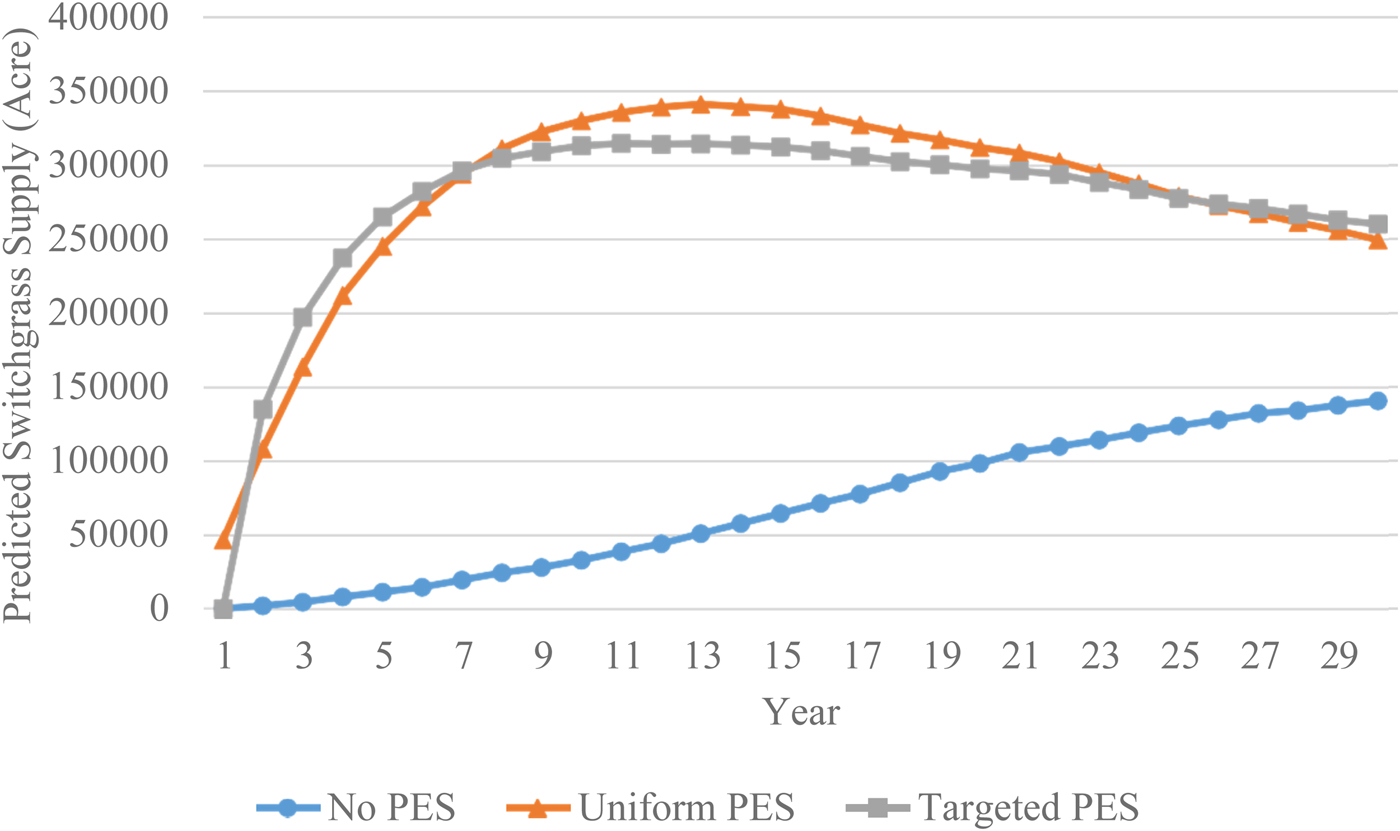
Figure 3. Predicted Land in Switchgrass: Segmented by Total Effectiveness
In general, the predicted land supply in switchgrass is much higher with both PES policies than with no PES policy. Of the two PES policies, in the short run (the first 1–8 years) the predicted land supply with the targeted PES policy is higher than the uniform PES policy. In the next period (Year 9–22), the uniform PES policy would generate higher land supply than the targeted PES policy with the peak of 341,006 acres in Year 13, while the peak for the targeted PES policy is 314,366 acres in Year 11. Both PES policies have a quite steady growth rate of land supply in switchgrass in this period, particularly during Year 10–20. In longer terms (Year 23–30), the growth rates slow down for both PES policies, and the land supply with the targeted PES policy again surpasses the uniform PES policy. Among the six groups, we observe that the predicted land supply in switchgrass of the TE The 4–5 group (nitrogen reduction rate 21.56 pounds/acre) is the highest in all three policy scenarios, followed by the TE 3–4 group (nitrogen reduction rate 16.77 pounds/acre) in the no PES and targeted PES scenarios, and the TE 1–2 group (nitrogen reduction rate 7.19 pounds/acre) in the uniform PES scenario.
Next, we use the predicted switchgrass land supply to estimate the potential nitrogen reduction. For each group the total nitrogen reduction in each year is calculated as the nitrogen reduction rate multiplied by the predicted land supply in switchgrass, and then the results are added up to obtain the aggregate nitrogen reductions. The aggregate results are shown in Figure 4. Both PES policy scenarios provide significantly higher nitrogen reduction than the no PES policy. The targeted PES policy provides higher nitrogen reduction than the uniform PES policy in all years, with the peak of 6,080,158 pounds in Year 10. We observe that the period with the highest nitrogen reductions for the targeted PES policy is Year 7–15, and for the uniform PES policy is Year 11–18. The nitrogen reduction grows slower for both PES policies after the first 15–20 years. Of the six groups, the TE 4–5 group (nitrogen reduction rate 21.56 pounds/acre) provides significantly more nitrogen reduction than the rest five groups.
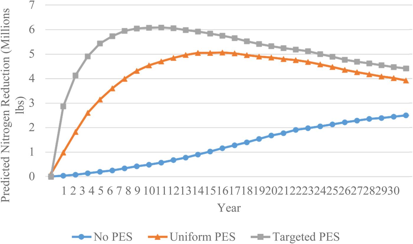
Figure 4. Predicted Nitrogen Reduction: Segmented by Total Effectiveness
The Monte Carlo simulation predictions suggest that the provision of PES can stimulate the land use conversion toward switchgrass, as we have discussed in the baseline model, and such policy effects become more significant in longer terms. Also, the targeted PES policy is shown to be more effective than the uniform PES policy with higher aggregate nitrogen reduction. While the uniform PES policy pays the same amount to all land parcels regardless of the relative different environmental performances, the targeted PES policy provides an optimized compensation scheme that can identify and prioritize the land use conversions on the land parcels that are the most effective in nitrogen reductions. Hence, the PES funds are more effectively used to stimulate land use conversion toward switchgrass in the high effectiveness land than in the low effectiveness land. However, future work should consider any potential differences in monitoring and implementation costs between targeted and uniform PES.
Moreover, according to the results, the PES policy is likely to be most effective in the first 10 to 20 years to incentivize the optimal switchgrass land and nitrogen reductions, but in longer terms the magnitude of the policy effects may decrease. This trend may be due to the life span of a switchgrass stand, which takes approximately 1 to 2 years to be established and may last 10 years with healthy production (Fike et al. Reference Fike, Parrish, Wolf, Balasko, Green, Rasnake and Reynolds2006). Beyond the normal life span, the switchgrass stand may decline in production and needs to be re-established, and the timing of the degradation of a switchgrass stand may vary due to the switchgrass cultivar, soil conditions and management techniques (USDA NRCS 2009). Hence, in longer terms the switchgrass supply may decrease as a result of losses in the previously established crops due to degradation, or conversion to other land use types after the switchgrass stand becomes less productive. To maintain an essential amount of switchgrass supply and nitrogen reductions in the long run, additional supplement policy programs may be necessary to help farmers replenish their switchgrass generations.
Furthermore, we compare the aggregated results of the three policy scenarios in Table 5. In particular, we look at the results in the years 10, 20, and 30, for comparisons of short term and long-term policy effects including predicted land supply in switchgrass, aggregate nitrogen reductions and total PES costs. Additionally, we compare the aggregate nitrogen reductions with Pennsylvania's targeted nitrogen reduction of 31.4 million pounds by 2025 (Pennsylvania State Government 2016). Overall, the policy effects of both PES policies significantly surpass that of the no PES policy, and the targeted PES policy performs better than the uniform PES policy in aggregate nitrogen reductions. Hence, the targeted PES policy may provide a more effective time path to achieve Pennsylvania's nitrogen reduction target than the uniform PES policy or no PES. Furthermore, the targeted PES policy provides nitrogen reductions at 8–19% lower cost per pound of nitrogen reduction.
Table 5. Comparisons of Policies: No PES, Uniform Payment, and Targeted PES by Total Effectiveness
Discussion
Perennial energy crops like switchgrass can potentially provide ecosystem services such as reducing the nutrient loading in watershed, but the current market supply may have been lower than expected partly due to the uncertainties related with the yields and economic returns of these crops. In this study, we use a dynamic optimization model for land use conversion to investigate the time-variant uncertainties that may affect the net returns of switchgrass, in comparison with the conventional corn-soybeans crop. As Song et al. (Reference Song, Zhao and Swinton2011) has discovered, by allowing a two-way conversion between switchgrass and corn-soybeans, farmers have the flexibility of making land use decision only based on the comparisons of their expectations of the NPV of chosen land use type in the foreseeable periods. Different from Song et al. (Reference Song, Zhao and Swinton2011) and other previous work, we offer farmers with monetary subsidies in the form of a PES policy to incentivize switchgrass supply. This PES policy is found to be effective in motivating land use conversions toward switchgrass, as in the short run the instantaneous switchgrass net return necessary to incur conversion from corn-soybeans is lower with the PES, and in the long run more land is used for switchgrass supply and more nitrogen reduction can be achieved. Switchgrass ethanol can also provide an abundant supply of energy while reducing the GHG emissions if it is used to replace the conventional fossil fuels, particularly in the aviation industry.
In addition, we extend the analysis by allowing the PES payments to vary according to the effectiveness of the crop land in terms of nutrient sequestration, and with the implementation of a targeted PES policy the results show improved results than the uniform PES policy as more land is used for switchgrass in the long run. In both the uniform and targeted PES policy scenarios, we have found significant nitrogen reductions as compared with the scenario of no PES, with the targeted PES policy generating the most nitrogen reductions. It should be noted that such high levels of environmental service would require large amount of abatement costs; hence, it is necessary that the regulators make the tradeoff between the budget and efficiency of the PES policy choices.
Our results suggest that the application of a PES policy or other monetary supplements to farmers can stimulate agricultural land use conversions toward perennial energy crops and promote the market supply, thus correcting the market failure of undersupply of these crops when no policies are implemented. To efficiently compensate farmers for the environmental performances and to optimize the perennial energy crop in the long run, information of the agricultural land such as the effectiveness in generating environmental benefits such as nutrient sequestration is needed. Indeed, by applying our simulations on predictions of the long run land use conversions in Pennsylvania, we have discovered that land of different effectiveness levels show different trends of long run switchgrass supply. Moreover, the longevity of the energy crop species among other factors may also affect the effects of the PES policy particularly in longer terms, usually beyond the 20-year period. Thus, future studies may extend our results by determining the optimal length of the PES policy and the evaluating the variations of the policy effects in the long run due to factors that may affect switchgrass production and market fluctuations. Furthermore, future work could also consider PES contracts that require longer term commitments to switchgrass production, such as contract lengths of five to ten years.
Acknowledgments
This work was supported by the Aviation Sustainability Center (ASCENT) – the Federal Aviation Administration’s (FAA) Center of Excellence for Alternative Jet Fuels and Environment – with funding under Award Number 13-C-AJFE-PSU-28. Any opinions, findings, and conclusions or recommendations expressed in this material are those of the authors and do not necessarily reflect the views of the FAA. This work was also supported by Department of Agricultural Economics, Sociology, and Education at the Pennsylvania State University and the USDA National Institute of Food and Agriculture and Multistate Hatch Appropriations under Project # PEN04631and Accession # 1014400. The authors would like to thank Tom Richard and Armen Kemanian at Penn State for their support throughout the project, Jeff Sweeney at the United States Environmental Protection Agency for his help with the relative effectiveness of nitrogen reduction throughout the Chesapeake Bay, Laurence Eaton at the Oak Ridge National Lab for providing the switchgrass returns data, and Feng Song at Renmin University, Beijing, China and Scott Swinton at Michigan State University for sharing their code to estimate the dynamic optimization land use conversion model. We would also like to acknowledge helpful comments from audience members at the FAA ASCENT annual meetings, the Northeastern Agricultural and Resource Economics Association annual meetings, and the Agricultural and Applied Economics Association annual meetings. All data are publicly available (see Estimation and Data section and citations therein for details).
APPENDIX: Net Present Value vs. Dynamically Optimal Conversion Boundaries
(1) TE 0–1 Group
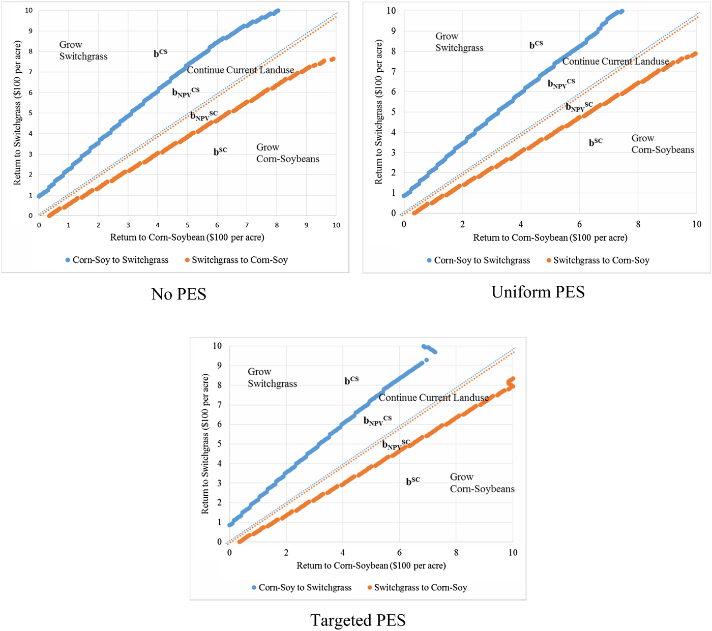
(2) TE 1–2 Group
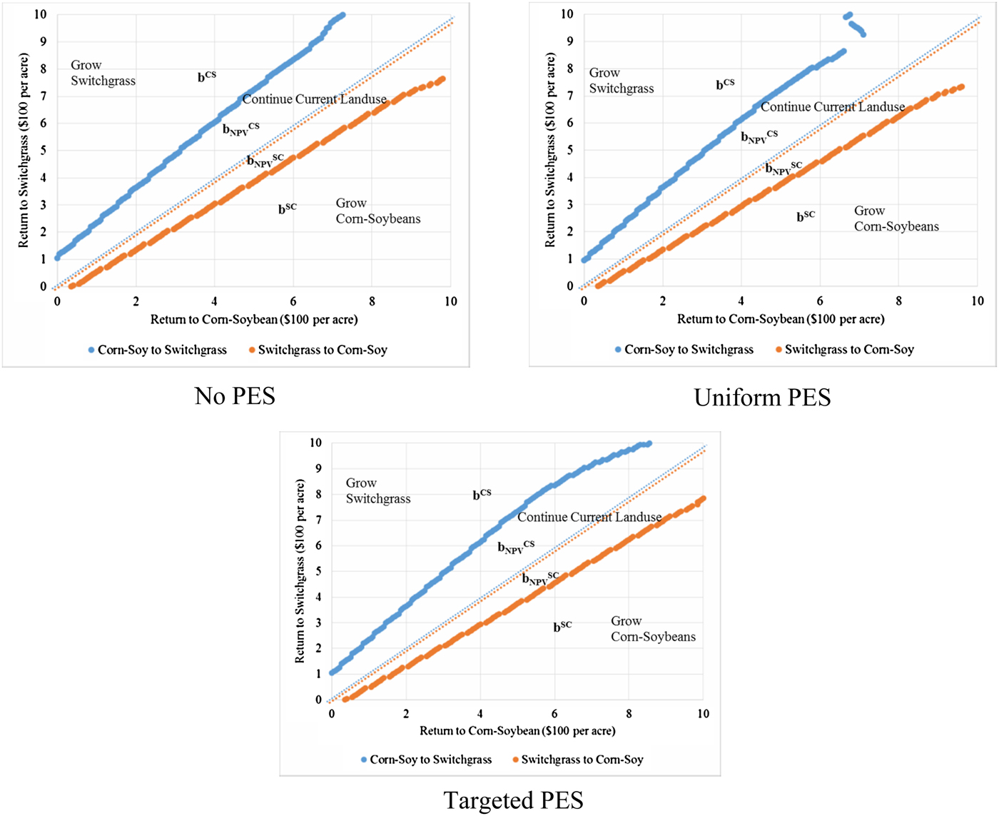
(3) TE 2–3 Group
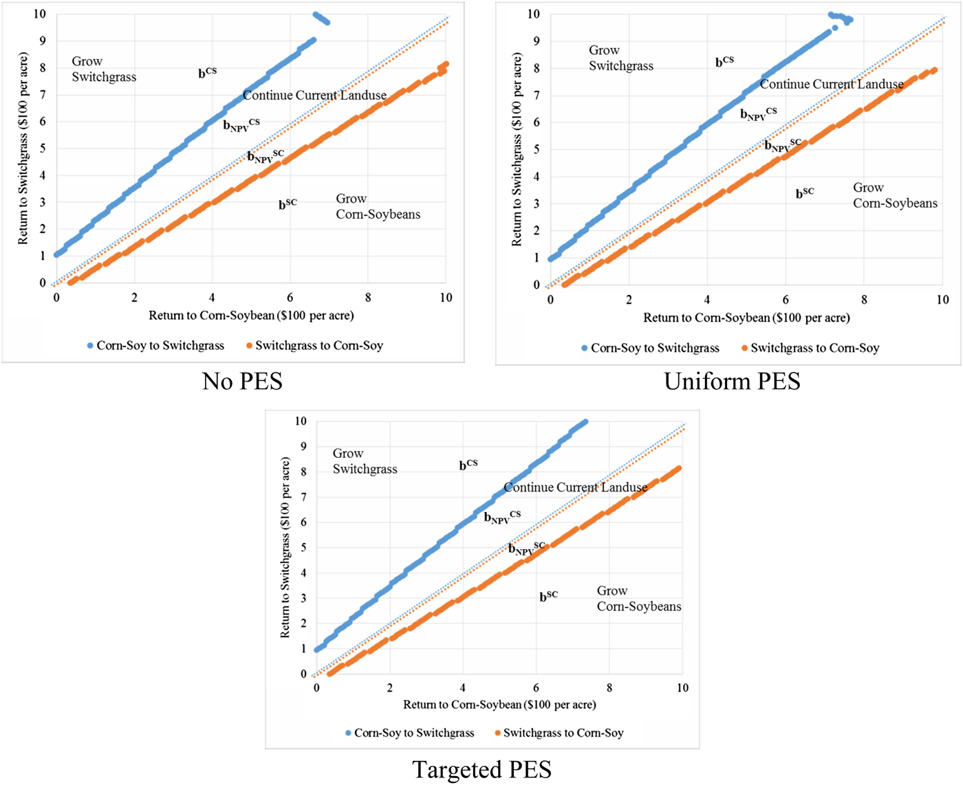
(4) TE 3–4 Group
(5) TE 4–5 Group
(6) TE Above 5 Group


 Open access