


Introduction
Discrete choice experiments are frequently used to collect data that facilitates understanding of consumer preferences. Best-worst scaling (BWS), first used by Finn and Louviere to study food safety (Finn and Louviere Reference Finn and Louviere1992), is one type of discrete choice experiment that results in the relative ranking of product attributes. BWS scaling involves presenting respondents with subsets of attributes drawn from a larger total set, and asking them to select the best and worst, the most important and least important, etc., from the subset provided to them. These combinations of subsets are defined as choice scenarios, and several choice scenarios are required to establish the continuum of rank. The combination of the number of attributes per choice scenario and number of choice scenarios in a given design is statistically determined, and researchers often have several design options with the same statistical power as measured by efficiency (Johnson et al. Reference Johnson, Lancsar, Marshall, Kilambi, Mühlbacher, Regier, Bresnahan, Kanninen and Bridges2013). BWS has advantages over other ranking methods, such as Likert scales, because the method forces respondents to make trade-offs (Lusk and Briggeman Reference Lusk and Briggeman2009). Additionally, when using BWS, numbers are not associated with the ranking, which avoids the issues of respondents assigning different values to numbers as well as cultural differences between numbers when conducting international studies (Auger, Devinney and Louviere Reference Auger, Devinney and Louviere2007).
Until recently, little discussion has surrounded the possible impact of BWS design choice on data collected. Byrd et al. (Reference Byrd, Widmar and Gramig2018) found differences in relative rank and preference share size of the attributes between two BWS designs. The two designs included the same six attributes, but one design presented respondents with two attributes per choice scenario for a total of fifteen choice scenarios, while the other design presented respondents with three attributes per choice scenario for a total of ten choice scenarios. Although there were differences found between the two different designs it is not possible to determine if the differences resulted from the number of attributes or choice scenarios presented to the respondent, or both.
Studies have shown that long surveys can cause fatigue, which may result in poor data quality (Galesic and Bosnjak Reference Galesic and Bosnjak2009). For longer surveys, responses to open-ended questions were shorter, response rates for individual questions decreased, and there was less variability in grid type questions (Galesic and Bosnjak 2019). Choice experiments, including but not limited to BWS experiments, are often included as part of a longer survey instrument. A full factorial design for a BWS experiment would include every possible combination of attributes, and the continuum of preference would be determined by the respondent’s choices (Louviere, Flynn and Marley Reference Louviere, Flynn and Marley2015). Due to length constraints, it is impractical to use the full factorial design, so researchers employ a partial factorial method often designed using readily available software programs (Flynn Reference Flynn2010), such as the SAS %MktBSize macro (SAS 2018).
Statistical efficiency means that in large samples, if the distribution tends toward normality, the statistic has the least probable error (Fisher Reference Fisher1922). Response efficiency is the measurement error that results from cognitive effects that result in inattention to choice questions or unobserved contextual influences (Johnson et al. Reference Johnson, Lancsar, Marshall, Kilambi, Mühlbacher, Regier, Bresnahan, Kanninen and Bridges2013). Researchers are often forced to make trade-offs between statistical efficiency and response efficiency. Cognitive effects that result in poor-quality responses in discrete choice experiments can include simplifying heuristics (Johnson et al. Reference Johnson, Lancsar, Marshall, Kilambi, Mühlbacher, Regier, Bresnahan, Kanninen and Bridges2013; Alemu et al. Reference Alemu, Mørkbak, Olsen and Jensen2013; Scarpa et al. Reference Scarpa, Zanoli, Bruschi and Naspetti2012), respondent fatigue (Johnson et al. Reference Johnson, Lancsar, Marshall, Kilambi, Mühlbacher, Regier, Bresnahan, Kanninen and Bridges2013; Galesic and Bosnjak Reference Galesic and Bosnjak2009; Day et al. Reference Day, Bateman, Carson, Dupont, Louviere, Morimoto, Scarpa and Wang2012), confusion or misunderstanding (Johnson et al. Reference Johnson, Lancsar, Marshall, Kilambi, Mühlbacher, Regier, Bresnahan, Kanninen and Bridges2013; Day et al. Reference Day, Bateman, Carson, Dupont, Louviere, Morimoto, Scarpa and Wang2012), and inattention resulting from hypothetical bias (Johnson et al. Reference Johnson, Lancsar, Marshall, Kilambi, Mühlbacher, Regier, Bresnahan, Kanninen and Bridges2013). Statistical efficiency can be improved by including a large number of difficult trade-off questions – the opposite of what improves response efficiency. Response efficiency improves by asking a smaller number of easier trade-off questions. Sample size also impacts statistical power: larger samples shrink the inverse of the square root of the sample size which results in smaller confidence intervals (Johnson et al. Reference Johnson, Lancsar, Marshall, Kilambi, Mühlbacher, Regier, Bresnahan, Kanninen and Bridges2013).
Considering choice experiment data quality in attribute non-attendance and transitivity
Simplifying heuristics are often associated with attribute non-attendance (ANA). ANA can occur when a respondent simplifies the choice task by ignoring an attribute, which is problematic because choice experiments are based on random utility theory, and ignoring an attribute may alter the marginal effect (Scarpa et al. Reference Scarpa, Zanoli, Bruschi and Naspetti2012). Methods to account for ANA, including stated and inferred ANA, have been widely used in the willingness-to-pay (WTP) literature (Carlsson et al. Reference Carlsson, Frykblom and Lagerkvisk2007; Napolitano et al. Reference Napolitano, Braghieri, Piasentier, Favotto, Naspetti and Zanoli2010; Olynk et al. Reference Olynk, Tonsor and Wolf2010). WTP can either increase or decrease when accounting for ANA (Layton and Hensher Reference Layton and Hensher2008). Inferred ANA requires the evaluation of individual respondent’s coefficients of variation, and employs a threshold to determine occurrences of ANA (Hess and Hensher Reference Hess and Hensher2010). Widmar and Ortega (Reference Widmar and Ortega2014) employed inferred ANA to determine the effects using different thresholds for stated ANA while evaluating WTP for various livestock production attributes for dairy and ham products. The different thresholds investigated in their study (1, 2, and 3) resulted in only small changes in the WTP estimates (Widmar and Ortega Reference Widmar and Ortega2014). Stated ANA requires an additional question asking respondents directly if they ignored any of the attributes included in the choice experiment (Hole Reference Hole2011). In addition to design choices that impact response efficiency, accounting for ANA may help improve data quality.
Discrete choice models, including BWS are rooted in random utility theory (Scarpa et al. Reference Scarpa, Zanoli, Bruschi and Naspetti2012; Johnson et al. Reference Johnson, Lancsar, Marshall, Kilambi, Mühlbacher, Regier, Bresnahan, Kanninen and Bridges2013). The axioms of consumer theory, including transitivity (Varian Reference Varian1978), can be used as one method of data quality evaluation in choice experiments. Transitivity implies that if A is preferred to B and B is preferred to C, then A must be preferred to C (Varian Reference Varian1978). Issues related to response efficiency, such as respondent fatigue, confusion or misunderstanding, and inattention potentially resulting from hypothetical bias may result in violations of transitivity. Lagerkvist (Reference Lagerkvist2013) found the possibility of transitivity violations in choice experiments, but did not determine the number of transitivity violations or violators. Bir (Reference Bir2019) developed a Python algorithm employing directed graphs to determine the number of violations of transitivity at the individual level in four BWS designs. Accounting for the number of transitivity violations and the impact of those violations on results is one way to evaluate data quality in choice experiments.
This article presents a new method of BWS data collection designed with the objectives of improving response efficiency and data quality. The new method strives to improve response efficiency by decreasing the number of choice scenarios required for completion by respondents while maintaining the total number of attributes studied. Minimizing the number of choice scenarios has been past achieved by increasing the number of attributes shown to respondents in each choice scenario within the BWS, or by decreasing the total number of attributes studied. The appeal to this new BWS data collection method is in allowing for a decreased number of choice scenarios while holding the number of attributes within a choice scenario constant, and without decreasing the number of attributes studied. The new method uses an initial filter question to determine the group of attributes drawn from a larger set that individual respondents do not find important. The respondent then participates in a tailored BWS design that does not include those, predetermined as unimportant, attributes resulting in a smaller experimental design overall. In aggregate, over the entire sample of respondents, the continuum of all attributes included in the study can be determined. This analysis employs the new BWS data collection method by eliciting consumer preferences for fluid dairy milk attributes. Results and measures of data quality are compared to the traditional method of BWS in terms of the size of preference shares, relative ranking of attributes by preference share, the number of incidences of ANA, and the number of incidences of transitivity violation and violators.
Materials and Methods
Consumer preferences for attributes of fluid dairy milk were used as a case study to compare results of the traditional BWS method to the new BWS data collection method. In BWS, respondents are asked to select the best or worst, most important or least important, most ethical or least ethical, etc. attribute from a subset of attributes presented (choice scenario; see Louviere, Flynn and Marley Reference Louviere, Flynn and Marley2015; Lusk and Briggeman Reference Lusk and Briggeman2009). The number of attributes presented in a choice scenario can vary and is statistically determined based on the number of attributes included in the experiment (Louviere, Flynn and Marley Reference Louviere, Flynn and Marley2015). In both BWS methods, respondents were presented with a series of choice scenarios. Within each choice scenario, respondents were asked to choose the most important and least important attribute (out of those attributes presented to them) when making a fluid dairy milk purchase. Nine attributes of fluid milk were included in this study: container material, rbST-free, price, container size, fat content, humane handling of cattle, brand, required pasture access for cattle, and cattle fed an organic diet. Most consumers are familiar with fluid dairy milk, which is important when introducing a novel methodological approach for data collection.
The survey instrument, designed to collect basic demographic information as well as the traditional BWS and the new BWS data collection method choice experiments, was distributed in April 2016 using Qualtrics, an online survey tool. Seven hundred and fifty respondents participated in the traditional and new BWS data collection methods. Lightspeed GMI, which hosts a large opt-in panel, was used to obtain survey respondents who were required to be 18 years of age or older. The sample was targeted to be representative of the US population in terms of gender, income, education, and geographical region of residence as defined by the Census Bureau Regions and Divisions (US Census Bureau 2015).
Respondents were randomly selected to participate in either the traditional BWS method first followed by the new BWS data collection method or participate in the new BWS data collection method first followed by the traditional BWS method (Figure 1). The two groups were designed to help mitigate, in aggregate, the potential for differences in the two methods due to order effects and also allowed for each respondent to participate in both methods. Therefore, when comparing the two methods, the subsamples were comprised of the same respondents who were presented the methods in different orders. The traditional BWS and new BWS data collection methods were compared by evaluating differences in preference share size, rank, number of incidences of ANA, and number of incidences of transitivity.
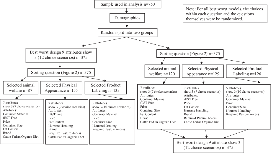
Figure 1. Survey design including sample size, and grouping of respondents.
Note: For all best worst models, the choices within each question and the questions themselves were randomized.
Traditional best-worst scaling method
The traditional BWS experiment was designed using the SAS %MktBSize macro which determines balanced incomplete block designs (SAS 2018). With nine attributes there were a total of five balanced designs to choose from. The number of attributes presented in a choice scenario ranged from three to eight and the number of choice scenarios ranged from nine to eighteen. The selected design presented respondents with three attributes per choice scenario, for a total of twelve choice scenarios. Each attribute appeared in the design 4 times.
Respondent choices were employed to determine the relative share of preference, or relative level of importance of each attribute. Each attribute’s location on the continuum from most important to least important was determined using the respondents’ choices of the most important and least important attributes from each choice scenario. The location of attribute j on the scale of most important to least important is represented by λ j . Thus, how important a respondent views a particular attribute, which is unobservable to researchers, for respondent i is:
 $${I_{ij}} = {\lambda _j} + {\varepsilon _{ij}}$$
where εij is the random error term. The probability that the respondent i chooses attribute j as the most important attribute and attribute k as least important is the probability that the difference between I ij and I ik is greater than all differences available from the available choices. Assuming the error term is independently and identically distributed Type I extreme value, the probability of choosing a given most/least important combination takes the multinomial logit form (Lusk and Briggeman Reference Lusk and Briggeman2009), represented by:
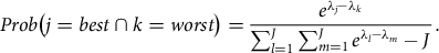 $$Prob\left( {j = best \cap k = worst} \right) = \displaystyle{{{e^{{\lambda _j} - {\lambda _k}}}} \over {\mathop \sum \nolimits_{l = 1}^J \mathop \sum \nolimits_{m = 1}^J {e^{{\lambda _l} - {\lambda _m}}} - {J^{\rm{}}}}}.$$
The parameter λ j , which represents how important attribute j is relative to the least important attribute, was estimated using the maximum likelihood estimation. To prevent multicollinearity one attribute must be normalized to zero (Lusk and Briggeman Reference Lusk and Briggeman2009).
A random parameters logit (RPL) model was specified to allow for continuous heterogeneity among individuals, following Lusk and Briggeman (Reference Lusk and Briggeman2009). The individual-specific parameter estimates from the RPL model were used to calculate individual-specific preference shares. The parameters are not directly intuitive to interpret, so shares of preferences are calculated to facilitate the ease of interpretation (Train Reference Train2009). The shares of preferences are calculated as:
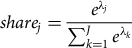 $$shar{e_j} = \displaystyle{{{e^{{\lambda _j}}}} \over {\sum\nolimits_{k = 1}^J {{e^{{\lambda _k}}}} }}$$
and must necessarily sum to one across the 9 attributes. The calculated preference share for each attribute is the forecasted probability that each attribute is chosen as the most important (Wolf and Tonsor Reference Wolf and Tonsor2013). Estimation was conducted using NLOGIT 6.0. The individual-level preference shares of the RPL model for each attribute were then averaged to represent the mean preference share of the sample. Standard deviations for the preference shares of each attribute were also determined in order to calculate confidence intervals for each preference share. Confidence intervals were calculated using the following formula:
 $$confidence\;interva{l_j} = mean \pm \left( {1.96*\left( \displaystyle{{{Standard\;Deviation} \over {SQRT\left( {Sample\;size} \right)}}} \right)} \right).$$
A 95% confidence interval was achieved by subtracting from the mean for the lower bound, adding for the upper bound, and using a z score of 1.96.
New best-worst data collection method
The objective of the new BWS data collection method was to institute a technique to establish a continuum from most important to least important attribute (in aggregate) while decreasing fatigue, through fewer choice scenarios and by decreasing the number of attributes included. The new BWS data collection method takes into account the idea that respondents each face attributes that will necessarily be at the bottom of their list of attributes ranked in importance.
According to Train (Reference Train2009), the logit probability for an alternative is never exactly zero. This is clear when considering the equation for the logit choice probabilities (equation 2). When λ i decreases, the exponential in the numerator of equation 2 approaches zero as λ i approaches -∞ and the share of preferences approaches zero. Since the probability only approaches zero, and is never exactly zero, if the attribute has no chance of being chosen by the respondent, the researcher can exclude it from the choice set (Train Reference Train2009).
Similar to Bir et al. (Reference Bir, Delgado and Widmar2020)’s approach with choice experiments designed to facilitate estimation of WTP, the first question in the new method (Figure 2) was designed to determine the category of attributes the respondent finds least important. For the newly proposed experimental design, the 9 attributes were grouped into three attribute categories: animal welfare attributes (pasture access, humane handling), product labeling attributes (fat content, organic diet, rBST free, brand), and physical appearance attributes (container material, container size). Price remained independent of the categories and was included in all component BWS experimental designs due to its consistent importance in other studies (Harwood and Drake Reference Harwood and Drake2018; Bir et al. Reference Bir2019; Lusk and Briggeman Reference Lusk and Briggeman2009). After identifying their least important category of attributes, each respondent participated in a component BWS choice experiment that did not include the attributes from the category the respondent indicated was least important to them. Fundamentally, the respondent was able to efficiently opt-out of seeing attributes belonging to their self-reported least important category of attributes. Although the attributes included in this study resulted in three logical categories, the number of categories may differ in future work employing this method. Furthermore, the use of categories may not be necessary, as the same technique could be used at the individual attribute level, wherein respondents choose the single attribute or un-categorized multiple attributes they do not find important, depending on the expected sample size and number of attributes included in the study.
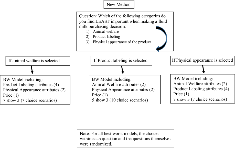
Figure 2. Flow of new best-worst data collection method including question prompt and options.
One of the benefits of the new BWS data collection method is that respondents answered fewer choice scenarios (the maximum number in this study was ten) when participating in the new BWS data collection method when compared to the twelve choice scenarios in the traditional method, while holding the number of attributes shown in each choice scenario constant at three. For the animal welfare and physical appearance attributes selected least important component BWS models, respondents completed seven choice scenarios. Each attribute appeared in a choice scenario three times for the animal welfare and physical appearance component BWS models. For the product labeling attributes selected least important component BWS model, respondents completed ten choice scenarios and each attribute appeared in a choice scenario 6 times. By intention, the three component BWS designs included different numbers of attributes. In order to combine the component BWS models, each component model (animal welfare attributes as least important model, product labeling attributes as least important model, and physical appearance attributes as least important model) was estimated separately and preference shares were calculated following equations 1–3. Once the preference shares for each individual were calculated, a preference share of zero was assigned to the attributes not included in the component model the respondent participated in, as determined by their selection of that category as least important. Using the same method as the traditional BWS, the average and standard deviation for each attribute’s preference share were calculated. Confidence intervals were calculated using equation 4. The overlapping confidence interval method (Schenker and Gentleman Reference Schenker and Gentleman2001) was used to determine if preference shares were statistically different within and between BWS models and methods.
Inferred attribute non-attendance
There are several ways to estimate inferred attribute non-attendance, for example, the equality-constrained latent class (ECLC) model uses a latent class logit model to identify ANA (Boxal and Adamowicz Reference Boxall and Adamowicz2002). The STAS model is another option for inferred ANA and is based on the Bayesian mixed logit model (Gilbride, Allenby and Brazell Reference Gilbride, Allenby and Brazell2006). In this study, incidences of inferred ANA were determined by calculating the coefficient of variation for individual respondent’s preferences for attributes and comparing them against a predetermined threshold (Hess and Hensher Reference Hess and Hensher2010). The coefficient of variation was calculated as:
 $$Coefficient\;of\;variation = \displaystyle\left| {{{individual\;standard\;deviation} \over {individual\;coefficient}}} \right|.$$
A threshold of 1 was used to determine incidences of ANA for the traditional BWS method. Widmar and Ortega (Reference Widmar and Ortega2014) evaluated thresholds of 1, 2, and 3 when evaluating inferred ANA in WTP choice experiments and found that the results were not very sensitive to the threshold chosen. A threshold of one was used in this analysis as a conservative choice. If the coefficient of variation exceeded the cutoff of 1, the attribute for that respondent was constrained to equal zero. As outlined by Greene (Reference Greene2012), the coefficients of the attributes were constrained to equal zero to signal values that were deliberately omitted from the data set by the individual respondent (Lew and Whitehead Reference Lew and Whitehead2020). The model was then re-estimated with incidences of ANA coded for each individual and each attribute. Individual preference shares were calculated, and the average, standard deviation, and confidence interval were calculated for each attribute using equations 3–4. For the new BWS data collection method, incidences of ANA were determined using a threshold of 1 within the component BWS models individually. Each new method component BWS model was re-estimated with the incidences of ANA coded, individual respondents were assigned preference shares of zero for attributes depending on the component BWS model they participated in, and averages, standard deviations, and confidence intervals for the aggregate of the component models were calculated using equations 3–4.
Transitivity violations
The frequency of transitivity violations was determined for both the new BWS and traditional BWS methods. The number of transitivity violations was determined for each component model of the new method individually and then aggregated to determine the number of violations for the new BWS data collection method. Custom Python code which relied on directed graphs was employed by Bir (Reference Bir2019) to determine transitivity violations for each respondent.
A respondent’s true preferences are never known by the researcher, therefore it is not possible to always determine the exact number of transitivity violations that occur; at best a minimum and maximum number of possible transitivity violations can be reported. To compare between the new BWS data collection method and the traditional method, the number of violators as a percentage of respondents was calculated. For the traditional method and the aggregate new BWS data collection method, the number of respondents was the same. However, the number of respondents differed between the three component BWS models of the new BWS method, and expressing the violators as a percentage allowed for statistical comparisons.
The number of potential violations differed between the new BWS and traditional methods, thus the number of possible violations per model was calculated as the number of choice scenarios multiplied by the number of respondents who participated in that model. For example, the animal welfare selected least important model consisted of 7 choice scenarios, and 207 respondents participated in this model, so there was a total number of possible violations of 1,149. The number of possible violations was summed across the three component BWS models to determine the total number of possible violations for the new BWS method model. The percentage of violations and violators were statistically compared using the test of proportions. In order to evaluate the impact of transitivity violators, and to compare their impact on preference shares to the uncorrected models, all models were re-estimated, as outlined in the above sections, with transitivity violators removed. Respondents who had at least one transitivity violation were considered a violator for the purposes of this analysis.
Results
Seven hundred and fifty respondents participated in both the traditional BWS method experiment and the new BWS data collection experiment. Table 1 includes the demographics from the US census in the first column, followed by the percentage of all respondents from the data collection. Since respondents could self-select into the categories for the new method, we reported the demographics for the three branches of the new method, animal welfare selected least important, physical appearance selected least important, and product labeling selected least important. Demographics between the self-sorted groups were statistically compared, and lack of statistical differences was indicated by matching letters as described in the table. Demographics between the self-sorted least important attribute subsamples differed (Table 1). A higher percentage of males (49%) selected animal welfare as least important when compared to the physical appearance and product. A lower percentage of respondent aged 25–34 (12%) were in the group physical appearance selected least important. For those who selected animal welfare least important, there was a lower percentage of respondents aged 45–54 (15%). A lower percentage of respondents aged 66 and older (18%) selected physical product labeling as least important when compared to animal welfare and physical appearance.
Table 1. Demographics of US census, entire sample, respondents who selected animal welfare as least important, physical appearance as least important, and product labeling as least important with statistical comparison between subsamples for demographics
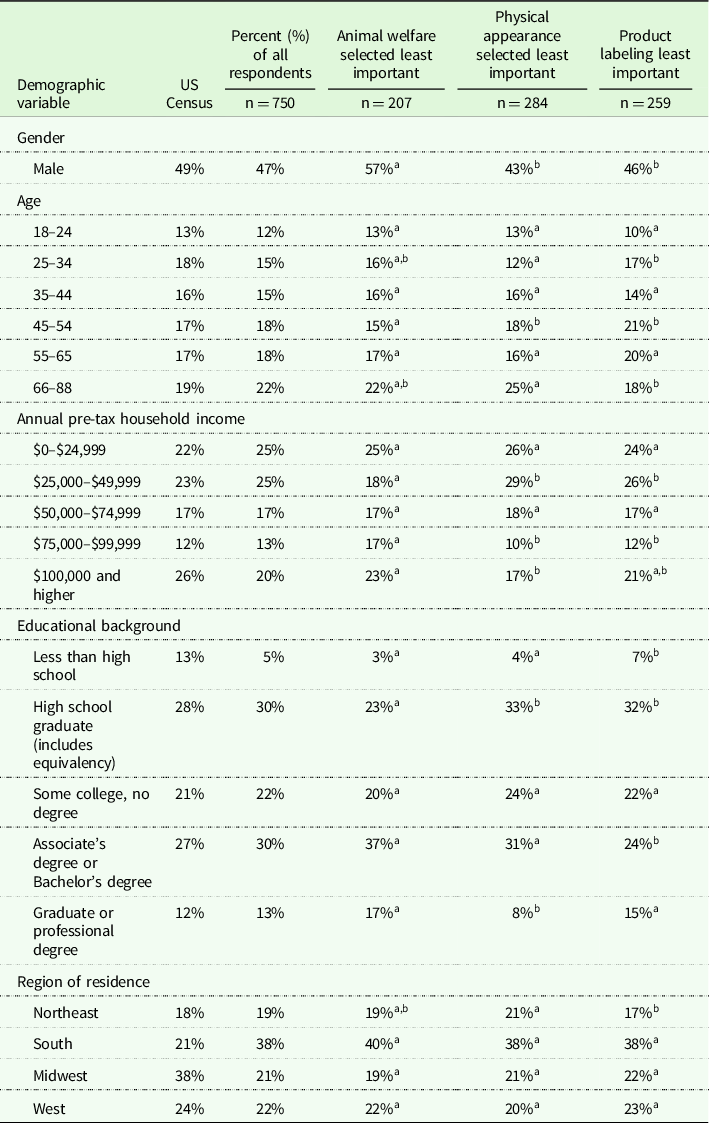
Matching letters indicate that demographic is not statistically different between the three self-selected categories animal welfare, product labeling, and physical appearance selected as least important. For example, the percentage of males is statistically different between animal welfare and product labeling and animal welfare and physical appearance, but is not statistically different between product labeling and physical appearance.
A lower percentage of respondents with an income of $25,000–$49,999 selected animal welfare as least important. Conversely, for respondents with an income of $75,000–$99,999 a higher percentage of respondents (17%) selected animal welfare as least important when compared to the physical appearance and product labeling. For respondents with an income of $75,000–$99,999 a higher percentage selected animal welfare as least important when compared to physical appearance. Lower percentages of respondents with less than a high school education (7%) and an associate’s degree or bachelor’s degree (24%) selected product labeling as least important. Lower percentages of respondents with a graduate degree or professional degree (8%) selected physical appearance, and lower percentages of high school graduates (23%) selected animal welfare as least important.
Traditional and new BWS data collection methods
Table 2 includes the RPL results and preference shares for both the traditional and new best-worst scaling collection method. The first column indicates the attributes included in the study. This is followed by the coefficients, standard deviation, and shares of preference for the traditional method (n = 750). Note these are the results before any corrections for transitivity violations or ANA have been made. This section is followed by the three columns that in combination are the new method results. The second section of the table includes two columns indicating the coefficients and standard deviation for the model of respondents who selected animal welfare as least important. This is followed by the coefficients and standard deviations for the model where physical appearance was selected most important, and product labeling as least important model results. The final column of the table indicates the preference share for the new best-worst data collection method, which is derived from the results of the three sub-models. Table 3 includes the confidence intervals (lower bound, mean, and upper bound) for the preference shares for both the traditional method and the new best-worst method. The first section depicts the original analysis. The preference share rank as determined by the overlapping confidence interval method is presented after the upper bound. At the end of the table, it is indicated if the models had preference shares that were statistically different in size as determined by the overlapping confidence interval method. The second set depicts the traditional method and new best-worst scaling method corrected for ANA; the preference share confidence interval and rank are given. After the rank column, a column indicates if the size of the preference share between the model with and without ANA correction is statistically different for each attribute. This column is available for both the traditional and new methods. The final column indicates if the ANA-corrected traditional method and if the ANA-corrected new method have statistically differing preference shares. The final models presented in table three are the traditional method and new method analyzed without transitivity violators. Columns are present to indicate statistical differences between the transitivity-corrected and nontransitivity-corrected, as well as between the new and traditional methods.
Table 2. RPL results and preference shares traditional method and new best-worst data collection method. Second and 3rd columns are the coefficients for the traditional method, column 4 are the preference shares. Columns 5 through 10 indicate the coefficients of the individual models that make up the new best-worst data collection method, with the last column indicating preference shares for the new method
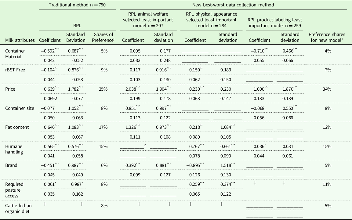
1 Calculated using the average of all individual respondent coefficients.
2 Crossed out boxes were not included in that BWS design.
* 1% Significance of coefficient.
┼ Dropped to avoid multicollinearity.
** 5% Significance of coefficient.
*** 1% Significance of coefficient.
Table 3. Confidence intervals of preference shares for traditional method and new best-worst data collection method given in column. The first grouping is the original model, second grouping is ANA-corrected, and third grouping is estimated without transitivity violators. Statistical difference indicated by yes/no
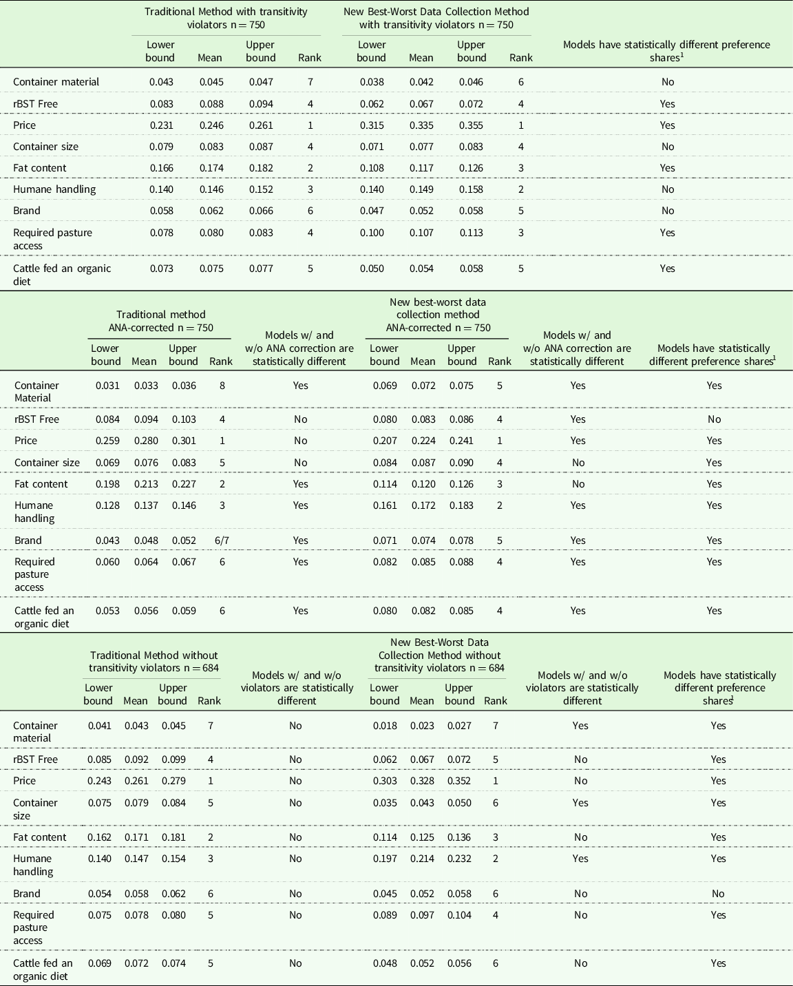
1 Traditional method and New Best-Worst Data Collection method have statistically different preference shares based on overlapping confidence intervals for either uncorrected, ANA-corrected, or transitivity-corrected model.
For both the uncorrected (for either transitivity violations or ANA) traditional and new BWS data collection methods the top attribute (price) and the bottom attribute (container material) were the same (Tables 2 and 3). However, the size of the preference share for price in the uncorrected new BWS data collection method was statistically higher than the traditional method. There was not a statistical difference in the size of the preference share for the lowest ranked attribute (container material) between the two methods. There were differences, in terms of order of attributes and size of preference shares, between the uncorrected traditional and new BWS data collection methods for the middle-ranked attributes. For the traditional method, the maximum number of ties in rank, as determined by overlapping confidence intervals, is three, which occurred once. For the new BWS data collection method, the maximum number of ties in rank was two, which occurred three times. The relative order between the two methods differed for fat content, humane handling, required pasture, cattle fed an organic diet, and brand. The size of the preference shares differed for rBST free, fat content, required pasture access, and cattle fed an organic diet.
Data quality comparisons between data collection methods
Table 4 indicates the number and percentage of both ANA occurrences and transitivity violations. The first section of the table indicates the number of ANA occurrences that occurred for each attribute. For example, the second column indicates the number of ANA occurrences that occurred for each attribute for the traditional method. The percentage of respondents who had an ANA occurrence was also calculated. So for example, for the traditional method 229 respondents (30.5%) had an ANA occurrence for container material. The next 3 columns in this section of the table indicate the number of respondents who had an ANA occurrence for the component models that make up the new best-worst scaling method. The final column indicates the total number of ANA occurrences (a summation of the component models), and the percentage of respondents for the new best-worst data collection method. The percentage of respondents with ANA occurrences were statistically compared between the traditional and new method and indicated in the table.
Table 4. Number of ANA transitivity occurrences for each attribute for the traditional and new best-worst data collection method. Number of transitivity violations and violators. Total number of minimum violations and percentage of violations, maximum number of violations and percentage of violations, final row indicates number of violators
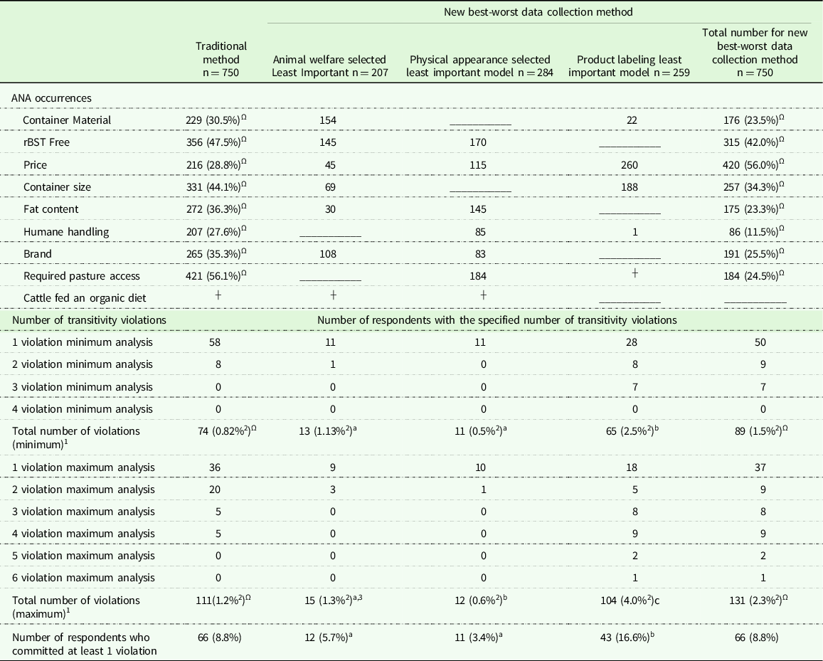
1 A respondents true preference is unknown by the researcher, therefore in some cases the number of possible violations is ambiguous. Therefore, the minimum and maximum number of violations is given.
2 Percentage calculated out of total number of opportunities for violation (calculated as the number of respondents multiplied by number of choice scenarios) from left to right: 9000,1149, 1988, 2590, 5727.
3 Matching letters indicates the percentage of violations or violators is not statistically different between the new method sub-models, differing letters indicate they are statistically different across the row.
┼ dropped to avoid multicollinearity.
Ω The percentage of ANA incidences or transitivity occurrences is statistically different between the traditional and new method.
When comparing the percentage of respondents who exhibited ANA between the traditional and new BWS data collection methods, for every attribute with the exception of price, higher percentages of respondents exhibited ANA while participating in the traditional method (Table 4). The ANA-corrected traditional method was statistically different in terms of size of preference share for all attributes with the exception of: rBST free, price, and container size when compared to the uncorrected traditional method (Table 3). The ANA-corrected new BWS data collection method differed from the uncorrected new BWS data collection method in terms of size of preference share for all attributes with the exception of container size, and fat content. The size of attributes preference shares differed between the ANA-corrected traditional method and the ANA-corrected new BWS data collection method for all but one attribute, rBST free. Similar to the results of the uncorrected methods, despite difference in the size of preference shares, the highest ranked attribute (price) was the same between the two ANA-corrected methods, and the lowest ranked attribute (container material) was the same between the two ANA-corrected methods. However, for the ANA-corrected new BWS data collection method there was a tie for last between container material and brand. Rankings differed between the ANA-corrected traditional and ANA-corrected new BWS data collection method for all attributes with the exception of price, rBST free, and container material. Both ANA-corrected methods had a maximum number of three ties, and the ANA-corrected new BWS data collection method had an additional tie between two other attributes.
Table 4 indicates the number and percentage of transitivity violations. Recall that the exact number of transitivity violations is unknown, because true preferences are unknown. Therefore, a minimum and maximum number of violations were determined for each individual. The minimum number of violations ranged from 1 to 4 across the three methods studied. The first column indicates the number of violations for the traditional method model. The first 4 rows of this section indicate the minimum number of violations. The 5th row indicates the total number of minimum violations and the percentage of violations. The percentage of violations is determined based on the total number of opportunities for a violation. This is calculated as the number of respondents multiplied by the number of choice scenarios for that model. For example, for the traditional method 58 people had 1 violation, and 8 people had two violations. This results in a total number of violations of 74 (58+(8*2)), which corresponds to 0.82% of total opportunities. Rows 6 through 11 indicate the maximum number of violations. For example, for the traditional method, 36 respondents had a maximum of 1 violation. Again, the total number of maximum violations as well as the percentage is given in the second to last row. The last row of the table gives the total number of respondents who committed at least one violation, as well as the percentage out of all respondent. For example, 66 respondents (8.8%) had at least 1 violation for the traditional method. To compare the number of transitivity violators across models, respondents who had at least a minimum violation number of 1 were indicated as violators. The same information is presented for the component models of the new best-worst scaling method in columns 3–5. The final column gives the totals for the best-worst scaling new method based on the component models.
The percentage of transitivity violators, defined as committing at least one transitivity violation, was not statistically different between the new BWS data collection method and the traditional method (Table 4). Interestingly only 10 respondents were violators in both the new method and the traditional method, which indicates the individual respondents committing violations were different in the two models. Shifting to analysis of the number minimum and maximum violations, the total number of violations was statistically higher in the new BWS data collection method when compared to the traditional method. Within the three new BWS component models, differences in the number of violations and the number of violators exists. The product labeling least important component model had a higher percentage of minimum violations, maximum violations, and violators when compared to physical appearance and animal welfare selected least important component models. Animal welfare selected least important and physical appearance selected least important had the same BWS design (show 3, 7 choice scenarios). Interestingly, the models did not differ significantly in the percentage of minimum violations and the percentage of violators.
Comparing the uncorrected traditional BWS model and the transitivity-corrected traditional BWS model, the relative rank changed for three attributes: cattle fed an organic diet, container size, and required pasture (Table 3). However, the size of the preference shares did not differ between the uncorrected and transitivity-corrected traditional models. For the new BWS data collection method, the relative rank also changed for three attributes-required pasture, container size, and brand, between the uncorrected and transitivity-corrected models. The size of the preference share between the uncorrected and transitivity-corrected new BWS data collection models differed for humane handling, container size, and container material. Interestingly, for all uncorrected and transitivity-corrected models, price was always ranked first and container material was always ranked last. There were many differences between the transitivity-corrected new BWS data collection method and the traditional method. With the exception of price and container material, the relative ranking differed for every attribute between the two transitivity-corrected models. Additionally, the size of the preference shares was statistically different between the transitivity-corrected models for all attributes, with the exception of brand.
Discussion
While participating in the new BWS data collection method, it was unsurprising that higher percentages of men self-selected animal welfare as least important when compared to the other categories. Female respondents exhibited increased concern for animal welfare in studies by Morgan et al. (Reference Morgan, Croney and Widmar2016), Vanhonacker et al. (Reference Vanhonacker, Verbeke, Van Poucke and Tuyttens2007), and McKendree et al. (Reference McKendree, Croney and Widmar2014). In a study of Finnish consumers, Yrjola and Kola (Reference Yrjola and Kola2004) found that respondents with lower incomes believed animal welfare was a more serious problem in Finnish agriculture. In a phone survey of US respondents, Prickett (Reference Prickett2008) found that those with a higher income were less likely to state they considered animal welfare at the grocery store. Conversely, Lagerkvist and Hess (Reference Lagerkvist and Hess2010) found in a meta-analysis that high income was a strong explanatory variable for consumer willingness-to-pay for farm animal welfare. In this study, there were only statistical differences in one of the lower income groups ($25,000–$49,999) and they were less likely to select that animal welfare was least important.
The results of BWS experiments are sensitive to the presentation of attributes, in terms of how many attributes are presented in a choice scenario (Byrd et al. Reference Byrd, Widmar and Gramig2018). This experiment accounted for those effects by employing only models with choice scenarios that included three attributes. When adjusting the number of attributes presented in a choice scenario between two and three, Byrd et al. (Reference Byrd, Widmar and Gramig2018) found that in terms of ranking, the top and bottom attributes were consistent between the two models. However, the size of the preference share for the attributes did change (Byrd et al. Reference Byrd, Widmar and Gramig2018). Note that due to the cardinal nature of preference shares, a change in preference share size is an important distinction (Wolf and Tonsor Reference Wolf and Tonsor2013). Given previous results found in the literature, it is perhaps unsurprising that between the new BWS data collection method and the traditional BWS collection method employed in this experiment, the top and bottom attributes did not change in terms of rank. Interestingly, for the attributes brand and container material which were in the bottom, or bottom two for both the traditional method and the new BWS data collection method-the preference shares were not statistically different across methods. This consistency exists even though 38% of respondents in the new BWS data collection method did not participate in a model with container material, 35% did not participate in a model with brand, and all respondents participated in fewer choice scenarios.
It is possible that the larger preference share for price resulting from the new BWS data collection method may be due to its appearance in all new BWS data component models. As previously stated, a logit probability for an alternative is never exactly zero (Train Reference Train2009). Therefore, the preference share for price was never exactly zero (the lowest for any individual respondent was 0.4%), unlike the other attributes which were set to zero if the respondent indicated they were not important. It is possible that price’s inclusion in all models may have resulted in an inflation of that particular preference share; however, the rank between the two methods for price did not differ, in both cases price was ranked solidly first. In further applications of this method, depending on the attributes included, it would be possible to include all attributes in a sorting question so that all attributes have the “opportunity” of being chosen as unimportant and therefore have a zero preference share. Further research could also compare and evaluate potential differences between selecting amongst grouped attributes as least important in comparison to selecting individual attributes. It is possible that some respondents may feel differently between the attributes that have been grouped together, and it is possible that not all studies include attributers which are easily and logically grouped.
Accounting for instances of ANA was one technique used to evaluate and compare the new BWS data collection method and the traditional method. It was hypothesized that because ANA may be caused by respondents simplifying choice tasks by ignoring attributes (Alemu et al. Reference Alemu, Mørkbak, Olsen and Jensen2013; Scarpa et al. Reference Scarpa, Zanoli, Bruschi and Naspetti2012) the new BWS data collection method may serve to lessen incidences of ANA. Fewer incidences of ANA did occur in the new BWS data collection method when compared to the traditional method. However, correcting for incidences of ANA still yielded results that were statistically different in terms of preference share size as well as attribute rank. It is possible that although there were fewer incidences of ANA in the new BWS data collection method, those remaining who exhibited ANA were particularly “bad offenders.” Bir et al. (Reference Bir, Delgado and Widmar2020) also found that the use of a filter question to decrease the number of questions respondents participated in decreased ANA for a WTP choice experiment. Additionally, they found that incidences of ANA were negatively correlated with the length of time respondents took to complete the experiment, which may lend credence to the idea of particularly bad inattentive offenders. The causes and implications of ANA in choice experiments, both BWS and willingness-to-pay, are unclear. Further studies are needed to determine what behavior is being captured when accounting for ANA, and whether this practice results in meaningful differences in results.
Consistent with the findings of Byrd et al. (Reference Byrd, Widmar and Gramig2018), and the ANA analysis in this experiment, despite correcting for transitivity violations the top (price) and bottom (container material) attributes in terms of relative ranking were immovable. Studying the same nine attributes for fluid dairy milk, price sorted to the top of the relative ranking and container material sorted to the bottom of the relative ranking for both Bir et al. (Reference Bir2019). The new BWS data collection had more statistically differently sized preference shares between the uncorrected and corrected for transitivity violation models when compared to the traditional BWS method. Despite this, correcting for transitivity resulted in a difference in relative ranking for three attributes in both methods, all occurring in attributes in the middle of the relative ranking. Given the novel nature of accounting for transitivity violators in BWS, it is unclear at this point how respondents who violate transitivity should be accounted for. Potentially, the first step is to begin regularly reporting transitivity violations as a metric of evaluation in BWS experiments. Perhaps in the future thresholds of acceptability could be developed either at the experiment or individual respondent level in regards to the number or percentage of transitivity violations.
When considering the component models of the BWS new data collection method, the product labeling selected as least important model appears to be the main driver of the higher number of transitivity violators and violations. It cannot be determined if the respondents who participated in the product labeling selected least important model were fundamentally different (recall this was a self-selected group), or if it was the particular design of the BWS experiment that resulted in the significant difference. The product labeling model resulted in 10 choice scenarios, which was higher than the animal welfare selected and physical appearance selected models. However, the traditional BWS method had 12 choice scenarios, and approximately half the number of violators in terms of percentage. Interestingly, the frequency of appearance for a given attribute was greatest for product labeling selected (6) when compared to the traditional method (4), and the animal welfare and physical appearance selected models (3). Further research is necessary to evaluate the impact that nuances in BWS experimental design choice result in beyond the number of attributes presented to respondents in a choice scenario or the number of choice scenarios.
Conclusion
A new BWS data collection method was introduced in this manuscript that builds on the traditional BWS method by decreasing the number of attributes shown to individuals and decreasing the number of choice scenarios required, while in aggregate allowing for the establishment of the continuum from least to most important for a larger number of attributes. The same set of respondents participated in both the new BWS data collection method and the traditional BWS method to determine the importance of nine different attributes when making a fluid milk purchase. The top (price) and bottom (container material) attributes in terms of relative ranking did not change between the new BWS data collection method and the traditional BWS method. Additionally, correcting for ANA and violators of transitivity did not impact the relative ranking of top and bottom attributes for either method. The relative ranking and size of preference share did differ between the new BWS data collection method, the traditional BWS method, and ANA/transitivity-corrected models. The new BWS data collection method resulted in fewer incidences of ANA for all attributes with the exception of one. However, there was no statistical difference in the number of transitivity violators between the new and traditional BWS methods.
The new BWS method provides researchers the opportunity to minimize the number of choice scenarios and attributes presented to respondents. The use of a filtering question to decrease the number of attributes included in individual respondent’s BWS experiments is a flexible contribution that can be adjusted to fit the attributes of the product studied. Different groupings of attributes or the selection of individual attributes as least important allow researchers to decrease the number of attributes and in turn the size of the experiment respondents participate in, while eliciting preferences for the larger set of attributes in aggregate. In longer, fatigue prone survey instruments the new BWS data collection method may be useful to minimize the number of questions presented to individual respondents while maintaining data quality. Data quality is measured here in terms of transitivity violations or ANA violations. Further research is needed to determine how the new BWS data collection method compares to the traditional method for other products and with varying BWS composite models for the new method.
Author contributions
CB, NW, and MD conceived and designed the analysis, wrote the paper. CB and NW collected the data. CB performed the analysis.
Funding statement
This work was funded, in part, by a Faculty Seed Grant provided by the Center for Animal Welfare Science at Purdue University in 2016. The funded project was entitled “Understanding Consumer Perceptions of Dairy Cattle Welfare.” Additional information can be found at https://vet.purdue.edu/CAWS/research.php. The funders had no role in study design, data collection and analysis, decision to publish, or preparation of the manuscript.
Conflicts of interest
The authors declare no conflicts of interest
Ethical standards
This work was approved by Purdue University IRB number 1703018932.


 Open access