

The forestry sector is sensitive to climate change, and it is likely that changing temperature and precipitation patterns will produce a strong direct impact on both natural and managed forests (Kirilenko and Sedjo Reference Kirilenko and Sedjo2007). On the one hand, climate change can accelerate vegetation growth with a warmer climate, longer growing seasons, and elevated atmospheric CO2 concentrations (Harsch et al. Reference Harsch, Hulme, McGlone and Duncan2009). On the other hand, climate change can increase the frequency and intensity of forest wildfires, insect and pathogen outbreaks, and shifting biomes (Scholze et al. Reference Scholze, Knorr, Arnell and Colin Prentice2006, Bachelet et al. Reference Bachelet, Lenihan, Drapek and Neilson2008, Gonzalez et al. Reference Gonzalez, Neilson, Lenihan and Drapek2010).
The way markets adapt to climate change-induced changes in forest growth and dieback will have important effects on projections of timber outputs, forest stocks, and the carbon stored in forested ecosystems. A number of bio-economic models have been developed to capture ecological impacts and to assess the potential economic effects of climate change on the forestry sector (e.g., Joyce et al. Reference Joyce, Mills, Heath, David McGuire, Haynes and Birdsey1995, Sohngen and Mendelsohn Reference Sohngen and Mendelsohn1998, Sohngen, Mendelsohn, and Sedjo Reference Sohngen, Mendelsohn and Sedjo2001; Perez-Garcia et al. Reference Perez-Garcia, Joyce, David McGuire and Xiao2002; Hanewinkel et al. Reference Hanewinkel, Cullmann, Schelhaas, Nabuurs and Zimmermann2013; Tian et al. Reference Tian, Sohngen, Kim, Ohrel and Cole2016; see Appendix 1). These studies show that climate change will tend to increase timber supply, reduce global timber prices, and change the incentives to manage forests. However, these existing studies have studied climate effects only through 2100 and so cannot predict long-term outcomes or the effects of higher temperature increases. Given the history of global mitigation to date, it is not likely that climate will be stabilized before 2100. It is therefore imperative to examine possible warming scenarios that extend beyond 2100 to both understand long-run timber implications and to explore possible climate scenarios that are far more severe.
This study examines the high-emission IPCC scenario associated with the representative concentration pathway (RCP) scenario that leads to 8.5 W/m2 radiative forcing (Riahi et al. Reference Riahi, Rao, Krey, Cho, Chirkov, Fischer, Kindermann, Nakicenovic and Rafaj2011). Combining this emission scenario with the HadGEM2 climate model (Martin et al. Reference Martin, Bellouin, Collins, Culverwell, Halloran, Hardiman, Hinton, Jones, McDonald, McLaren, O'Connor, Roberts, Rodriguez, Woodward, Best, Brooks, Brown, Butchart, Dearde, Derbyshire, Dharssi, Doutriaux-Boucher, Edwards, Falloon, Gedney, Gray, Hewitt, Hobson, Huddleston, Hughes, Ineson, Ingram, Pames, Johns, Johnson, Jones, Jones, Joshi, Keen, Liddicoat, Lock, Maidens, Manners, Milton, Rae, Ridley, Sellar, Senior, Totterdell, Verhoef, Vidale and Wiltshire2011) yields a severe warming scenario through 2300, with eventual temperatures that are 11 °C above 1900 levels. The RCP 8.5 scenario is compared to a (Baseline) scenario without climate change.
The dynamic ecosystem response is captured by the LPX-Bern global dynamic vegetation model (Stocker et al. Reference Stocker, Roth, Joos, Spahni, Steinacher, Zaehle, Bouwman and Prentice2013; Mendelsohn et al. Reference Mendelsohn, Prentice, Schmitz, Stocker, Buchkowski and Dawson2016). The LPX-Bern model predicts three changes in ecosystems as a result of climate change. First, the net primary productivity of vegetation will change, first rising and then (after 2150) stabilizing. Second, some of the standing stock will be lost to dieback from direct temperature effects and forest fires. Third, the distribution of biomes and timber species over space will change radically as species move poleward and to higher altitudes. All of this happens at particular dynamic rates that are part of the ecosystem model.
We then use five shared socioeconomic pathways (SSPs) (Riahi et al. Reference Riahi, van Vuuren, Kriegler, Edmonds, O'Neill, Fujimori, Bauer, Calvin, Dellink, Fricko, Lutz, Popp, Crespo, Samir, Leimbach, Jiang, Kram, Rao, Emmerling, Ebi, Hasegawa, Havlik, Humpenöder, Da Silva, Smith, Stehfest, Bosetti, Eom, Gernaat, Masui, Rogelj, Strefler, Drouet, Krey, Luderer, Harmsen, Takahashi, Baumstark, Doelman, Kainuma, Klimont, Marangoni, Lotze-Campen, Obersteiner, Tabeau and Tavoni.2017) that represent alternative growth rates of population and income to explore the consequence to future possible outcomes. The climate and ecosystem outcomes are examined using alternative socioeconomic projections to provide a full range of plausible outcomes for the timber market in the far future. Although the model does take into account how SSPs affect demand for timberland, the model is not well suited to study how SSPs might also change demand for farmland. This is a topic for future research.
An extended version of the global timber model (GTM) (Sohngen and Mendelsohn Reference Sohngen and Mendelsohn2003) is developed to study how the forest sector will respond to these future challenges. The timber model is a forward-looking model that examines what changes should be made in advance of all these future effects. For example, the model selects where to plant new trees under the future climate conditions. The model predicts increasing harvest rates of stands that have an ever-increasing rate of dieback. The model changes the intensity of management according to the future plants’ productivity by intensifying it in places that become more productive and reducing it in places that become less productive. Finally, the model forecasts future timber prices that will dictate the amount of forestland that will be managed and the amount of forestland that will remain natural (unmanaged).
The paper is organized as follows. Section “Methods” describes the method and the model used for the analysis. Section “Economic Results” analyzes the results of the model in terms of changes in timber market and forestland under the RCP 8.5 and compares them with the Baseline scenario (without climate change). Finally, Section “Conclusions” summarizes the results and discusses their implications.
Methods
Model
The GTM (Sohngen, Mendelsohn, and Sedjo Reference Sohngen, Mendelsohn and Sedjo2001; Sohngen and Mendelsohn Reference Sohngen and Mendelsohn2003; Favero and Mendelsohn Reference Favero and Mendelsohn2014) used in this study contains 200 forest types i in 16 regionsFootnote 1 that can be aggregated into four broad categories: boreal, temperate hardwood, temperate softwood, and tropical. The model assumes there is a social planner maximizing the present value of the net difference between consumer surplus and the costs of holding timberland and managing it over time. It is an optimal control problem, given the aggregate demand function, starting stock, costs, and changing growth functions of forest stocks. It endogenously solves for timber prices and the global supply of timber and optimizes the harvest of each age class, management intensity, and the area of forestland at each moment in time. GTM is forward looking with complete information.
We change the original GTM model to include time steps to the year 2350. We do not report the final time steps of the model because they are sensitive to the assumptions made about terminal conditions. We consequently only report the results to 2250. These results are sufficiently far in front of 2350 that they are no longer sensitive to the terminal conditions.
The problem is written formally as:
 $$\max \!\sum\nolimits_0^\infty \!\!{{\rm \rho} ^t} \Bigg\{\!{\int\limits_0^{Q_t^{^\ast}} \!\!{\lcub {D\lpar Q_t\comma \, Z_t\rpar - f\lpar Q_t\rpar } \rcub dQ_t} -\!\! \sum\limits_i {p_m^i m_t^i G_t^i - \!\!\sum\limits_i {C^i\lpar {N_t^i} \rpar } -\!\! \sum\limits_i {R^i\bigg(\!{\sum\limits_a {X_{a\comma t}^i}}\!\! \bigg)}}} \!\!\Bigg\}\comma \; $$
where ρ is a discount factor, D(Q t) is the global demand function for industrial timberFootnote 2, f(Q t) is the cost of harvesting and transporting timber to the mill, p m is the price of management intensity m, G t is planted acreage, C(N t) is the cost of new forestland N at time t, R(∑X a,t) is the opportunity cost of land X in age class a at time t. The objective function in (1) is nonlinear.Footnote 3 The model assumes that management intensity is determined at the moment of planting, and planting costs vary depending upon management intensity.
Timber demand Q t, is assumed to grow over time as the global economy grows:
 $$Q_t = A\lpar Z_t\rpar ^{\rm \beta} \lpar P_t\rpar ^{\rm \omega}\comma \; $$
where A is a constant, Z t is the projected global consumption per capita over time, β is the income elasticity, P t is the international price of wood, and ω is the price elasticity. To predict Z t ,we use the global consumption per capita from the SSPsFootnote 4 (see Section “Climate and Socioeconomic Scenarios”).
To determine the quantity produced in each region, the model chooses the age class to harvest trees. Thus, the total quantity harvested Q t will be obtained by summing the volume of timber on each hectare harvested in each age class and species type. The total timber area is tracked by the stock variable X a,t, and it adjusts over time. Timber shifts from one age class to the next unless harvests occur.
GTM takes into account the competition of forestland with farmland using a rental supply function for land (Sohngen and Mendelsohn Reference Sohngen and Mendelsohn2003). In Equation (1), R is the rental cost function for holding timberland X a,t. This supply function is restricted to farmland that is naturally suitable for forests according to the ecological model. It reflects the opportunity cost of agricultural rents lost when land is moved from farmland to forestland. It presumes that the forest will acquire the least productive farmland first in each region of the world.Footnote 5
We include in the forestry model three expected impacts of climate change as predicted by the LPX-Bern global dynamic vegetation model (DGVM): (a) changes in the net primary productivity (NPP) that measures the net carbon stored annually by an ecosystem; (b) changes in dieback; and (c) changes in the distribution of biomes and timber types. The LPX-Bern DGVM generates outputs at the 1° spatial resolution at a yearly time step. Outputs are then aggregated to decadal averages across world regions for use in the forestry model.
As in Sohngen, Mendelsohn, and Sedjo (Reference Sohngen, Mendelsohn and Sedjo2001), we assume changes in merchantable timber growth rates are proportional to predicted changes in NPP (θt) as predicted by LPX-Bern Model and management intensity, m t0. The changes in the timber volume V t are calculated as:
 $$V_t\lpar {m_{t0}^i\comma \; {\rm \theta}_t^i} \rpar = \int_{t0}^t {\mathop {V_s}\limits^ \bullet} \lpar {m_{t0}^i\comma \; {\rm \theta}_s^i} \rpar ds.$$
The forestry literature has examined the impact climate is expected to have on timber through 2100 (Sohngen, Mendelsohn, and Sedjo Reference Sohngen, Mendelsohn and Sedjo2001; Reilly et al. Reference Reilly, Paltsev, Felzer, Wang, Kicklighter, Melillo, Prinn, Sarofim, Sokolov and Wang2007; Buongiorno Reference Buongiorno2015; Tian et al. Reference Tian, Sohngen, Kim, Ohrel and Cole2016). However, warming that can happen through 2100 is quite limited so that no scenario has ever explored warming above 4 °C. By extending the timeline to 2250, this analysis will include both longer-term ecological effects and a climate scenario that reaches much higher temperatures. There is more time for higher cumulative emissions, higher temperatures, and more complete ecosystem responses.
We include the effect of dieback by using dieback rates from the DGVM, which affect all existing stocks of forest as follows:
 $$X_{a\comma t}^i = \lpar 1 - {\rm \delta} _t^i \rpar X_{a - 1\comma t - 1}^i - H_{a - 1\comma t - 1}^i + G_{a = 1\comma t - 1}^i + N_{a = 1\comma t - 1}^i\comma \; $$
where X is the area of land, H is the area of timberland harvested, G is the area of land regenerated, N is the area of new land established, and δ is the annual mortality rate from dieback from direct temperature effects and forest fires as predicted by the vegetation model. We assume that all age classes a have equal probability of dieback because the ecological model cannot predict which age classes are more vulnerable. Dieback also alters timber harvests H because some of the stock that dies back will be salvaged. The salvage enters the equation for net market surplus through harvests.Footnote 6
Finally, forest stock is also a function of the movement of biomes across the land. In this study, we include the changes in biomes due to climate change from the vegetation model. In the model, we separate the timber stocks into stocks that shift from one type to another during climate change and stocks which remain in their initial timber type. The distribution of biomes from the vegetation model is derived from the simulated vegetation composition and structure, following Prentice, Harrison, and Bartlein (Reference Prentice, Harrison and Bartlein2011). Initial forest stocks are given, and all choice variables are constrained to be nonnegative.
Climate and Socioeconomic Scenarios
The study compares the future potential climate impacts on global forests under the RCP 8.5 (Riahi et al. Reference Riahi, Rao, Krey, Cho, Chirkov, Fischer, Kindermann, Nakicenovic and Rafaj2011; van Vuuren et al. Reference Van Vuuren, Edmonds, Kainuma, Riahi, Thomson, Hibbard and Hurtt2011) with a no climate change scenario (Baseline). The CO2e concentrations in the RCP 8.5 rapidly rise to 1240 ppm by 2100 and to 1686 ppm by 2150, and then start to stabilize reaching 2222 ppm by 2300 (Meinshausen et al. Reference Meinshausen, Smith, Calvin, Daniel, Kainuma, Lamarque and Matsumoto2011). For this study we use a future climate projection from the climate model, HadGEM2. The RCP 8.5 concentration path is entered into HadGEM2 which predicts the future climate across the planet through 2300. The HadGEM2 model predicts that under the RCP 8.5 scenario global average temperature increases at a rapid rate through 2150 and then begins to slow down, stabilizing at 11 °C above 1900 by 2300.
The LPX-Bern DGVM is then used to simulate the vegetation response to climate change from the present to year 2300 (Mendelsohn et al. Reference Mendelsohn, Prentice, Schmitz, Stocker, Buchkowski and Dawson2016). As shown in Table 1, the increase in CO2 fertilization and warming during the twenty-first century under the RCP 8.5 scenario will increase forest productivity at the global level through 2150 compared to the Baseline. Beyond 2150, productivity stabilizes. On average the increase in forest productivity is greater in high latitude forests than low-mid latitude forests. As boreal forest is replaced by temperate forests, productivity rapidly increases. As shown in Table 1, under RCP 8.5, the absolute dieback rate is higher for high-latitude regions than low-mid latitude regions. However, dieback declines over time in the boreal and temperate regions, whereas it is more stable in tropical regions. For the Baseline scenario, we assume the dieback rate is fixed at the current (2010) level.
Table 1. (a) Projected percentage changes in NPP under the RCP 8.5 with respect to the baseline scenario; (b) Projected average dieback rate for each region under the RCP 8.5. Data from LPX-Bern global dynamic vegetation Model.

The ecosystem model also predicts that the share of each vegetation type will change over time. The changes under the RCP 8.5 scenario are dramatic as shown in Figure 1a. The boundaries of each biome shift with warming, causing some biomes to contract and others to expand. Overall, the potential of land available for forest will be reduced by 29 percent in 2150 and by 44 percent in 2250 relative to current levels. Forests are replaced by savanna, parkland, and woodlands, which contain only scattered trees and grassland. Potential tropical forests are relatively stable through 2150, declining by 17 percent and then shrinking by 32 percent in 2250. Boreal forests decline more rapidly, almost disappearing by the end of the 22nd century. Temperate and warm temperate forests grow through 2100 and then stabilize. Temperate forests often replace boreal forests in Canada, Europe, and Russia.
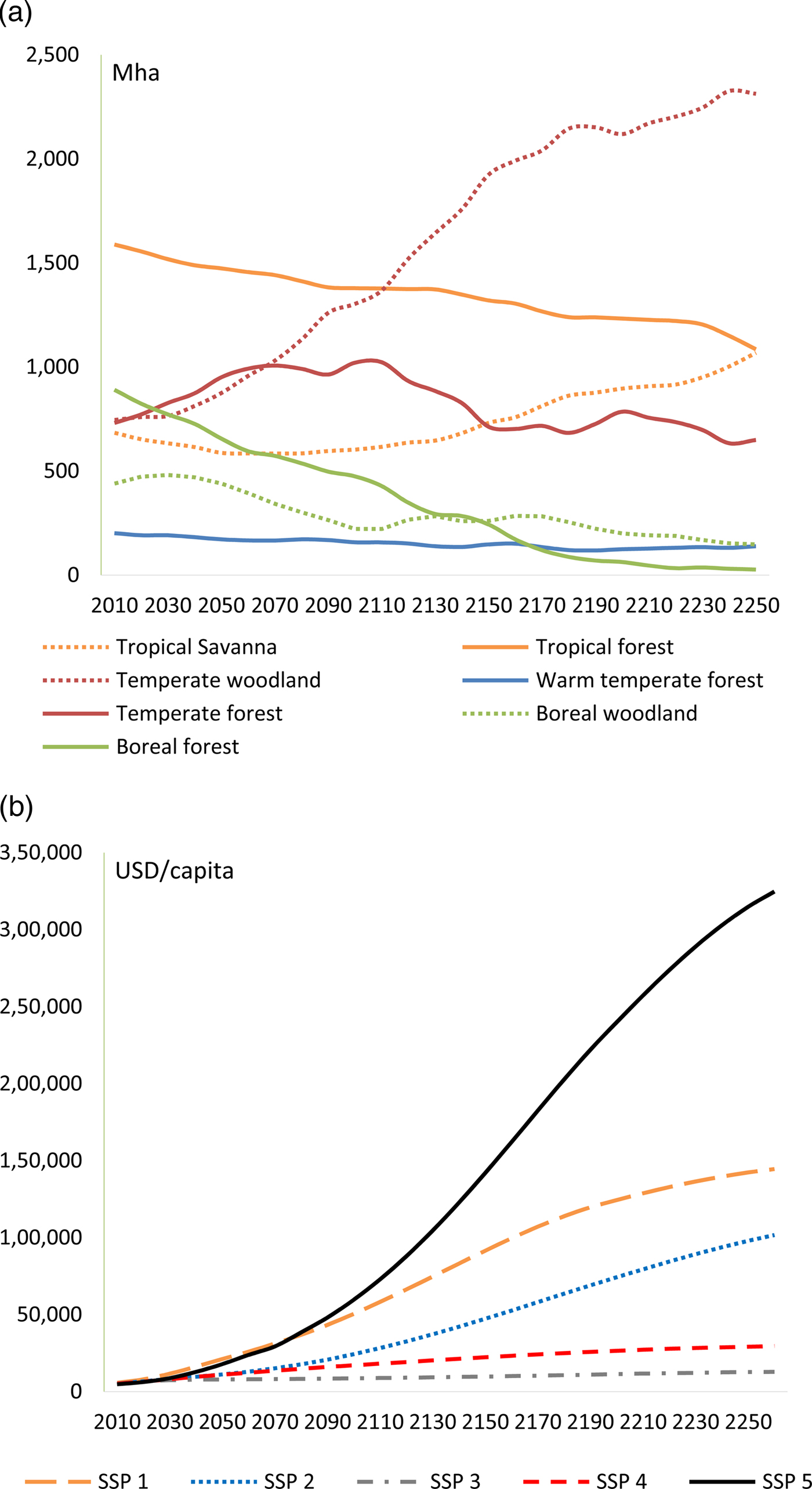
Figure 1. (a) Distribution of potential world vegetation under the RCP 8.5 scenario (Mha), data from LPX-Bern global dynamic vegetation model; (b) GDP per capita under the five socioeconomic scenarios.
Table 2 shows these forestland changes at the regional level. The changes under RCP 8.5 are dramatic for some countries: Russia, Europe, and the United States see the biggest losses of forestland in percentage terms. In Brazil forestland is projected to decrease by 55 percent relative to 2010 by 2250. The harm done in the Amazon is due to the strong drying that HadGEM2 predicts in the RCP 8.5 scenario. On the other hand, other regions are less affected or even gain forestland (Asia Pacific). For instance, in Southeast Asia, tropical forestland potential will increase at the expense of tropical savanna. Table 2 also reveals that there is not much forestland lost this century and that the biggest forestland losses occur in the 22nd century, when the change in global average temperature relative to preindustrial levels starts to exceed 8 °C.
Table 2. Percent change in potential forestland with respect to 2010 levels. Data from LPX-Bern Global Dynamic Vegetation Model

For both the RCP 8.5 scenario and the Baseline scenario, we use the 2010–2100 consumption and population from the five SSPs to calculate global consumption per capitaFootnote 7. Global consumption per capita drives global timber demand (see Z in Equation 2). In order to extend our analysis to 2300, we follow earlier analyses that assume continued-but-declining population growth beyond 2100, which finally stabilizes in 2200 (IAWG US, 2010). These assumptions lead to an S-shaped growth in population over time with a 2100 global population of 7–12.6 billion that then stabilizes. We also assume continued-but-declining economic growth rates reaching zero in 2300. This assumption also leads to an S-shaped growth in GDP over time (IAWG, 2010). By 2100, average global consumption has risen to $8,700–60,000 per capita and by 2250, consumption has risen to $12,700–315,000 per person, depending on the SSP (Figure 1b).
Economic Results
The increase in global per capita consumptions in the SSP1, SSP2, and SSP5 scenarios causes the demand for timber to increase over time in these socioeconomic scenarios. This increased demand for timber causes timber prices to rise, in order to supply more wood. The higher timber prices assure sufficient land is used to produce future timber and also to encourage more intensive land management. Managed forestland can potentially come from agricultural land or natural forest land. Of course, the higher timber prices also serve to temper demand.
In 2010, managed forestland accounts for 34 percent of total forestland. As the demand for timber increases under the SSP 1, SSP 2, and SSP 5, the amount of managed land increases, both in absolute and in relative terms. In 2250, under the Baseline scenario, the share of managed forestland increases to 36–41 percent depending on the SSPs. The most significant increase occurs under the SSP 5, when the dramatic increase in income requires more conversion of natural forests into managed forest: in 2250 the amount of managed forestland increases by 249 Mha, and the amount of natural forestland falls by 189 Mha (Table 3). The remaining 60 Mha of managed forestland came from marginal agricultural lands. The higher timber prices also increase management intensity, increasing supply. For instance, under the SSP 5, global average timber yield/ha will be about 50 percent higher than 2010 levels by 2100 and by 2250, it will be more than double.
Table 3. Global managed and natural forestland in (a) the Baseline scenario and (b) the RCP 8.5 Scenario.
The small increase in global consumption per capita under the SSP 3 and SSP 4 produces only a slight increase in the demand for timber. Under these scenarios, the increase in productivity outpaces the increase in demand and the price of timber rises only slightly and then starts to decline. As a result, under these two socioeconomic scenarios there is no incentive to convert additional land to managed forest, and the share of managed versus natural forest remains almost unaffected.
The picture changes under the RCP 8.5 climate scenario where global forests will experience (on average) a substantial gain in productivity. The managed forest no longer needs as much land as it did in the Baseline. The only scenario where managed land increases is in the SSP 5 scenario, and this increase is only temporary. So the RCP 8.5 scenario does not entail much land being shifted into managed forest and in fact becomes a source of land in most cases. It is the climate scenario itself that is taking a toll on natural forest. The HadGEM2 model predicts a shrinkage of global forest, all at the expense of the natural forest. In 2250, global forestland is reduced by 28–32 percent relative to the Baseline. Boreal forest almost disappears because of the ecosystem response to higher temperatures. Russia takes the largest hit and under SSP 5 loses 80 percent of its natural forest by 2250. However, the ecosystem model replaces a great deal of boreal forests with faster growing temperate forest. Most of this temperate forest will be managed. The ecological vegetation model predicts a large loss of natural tropical forest in the Amazon. This result is specific to the HADGEM2 climate model that predicts significant drying in the Amazon basin (Table 4).
Table 4. Regional changes in managed, natural and total forest under the RCP 8.5 relative to the Baseline scenario in 2250 (Mha)

Under the RCP 8.5 scenario, the large gain in forest productivity outweighs the loss in forest area. As illustrated by Figures 2 and 3, GTM predicts that global timber supply increases, and prices decline under all socioeconomic climate change scenarios relative to their correspondent baseline projections. Climate change causes global timber supply to increase by 19–24 percent above the Baseline by 2100. The results support the findings in the literature that climate change will increase timber output through 2100. The study reveals that this positive effect of climate change on timber supply continues through 2190 and then begins to slow (Figure 2a, b). The increasing timber supply from climate change leads to lower timber prices. The analysis supports earlier findings that climate change leads to lower timber prices through 2100. This effect continues through 2250 despite the very high temperatures associated with the 23rd century (Figure 3a, b).
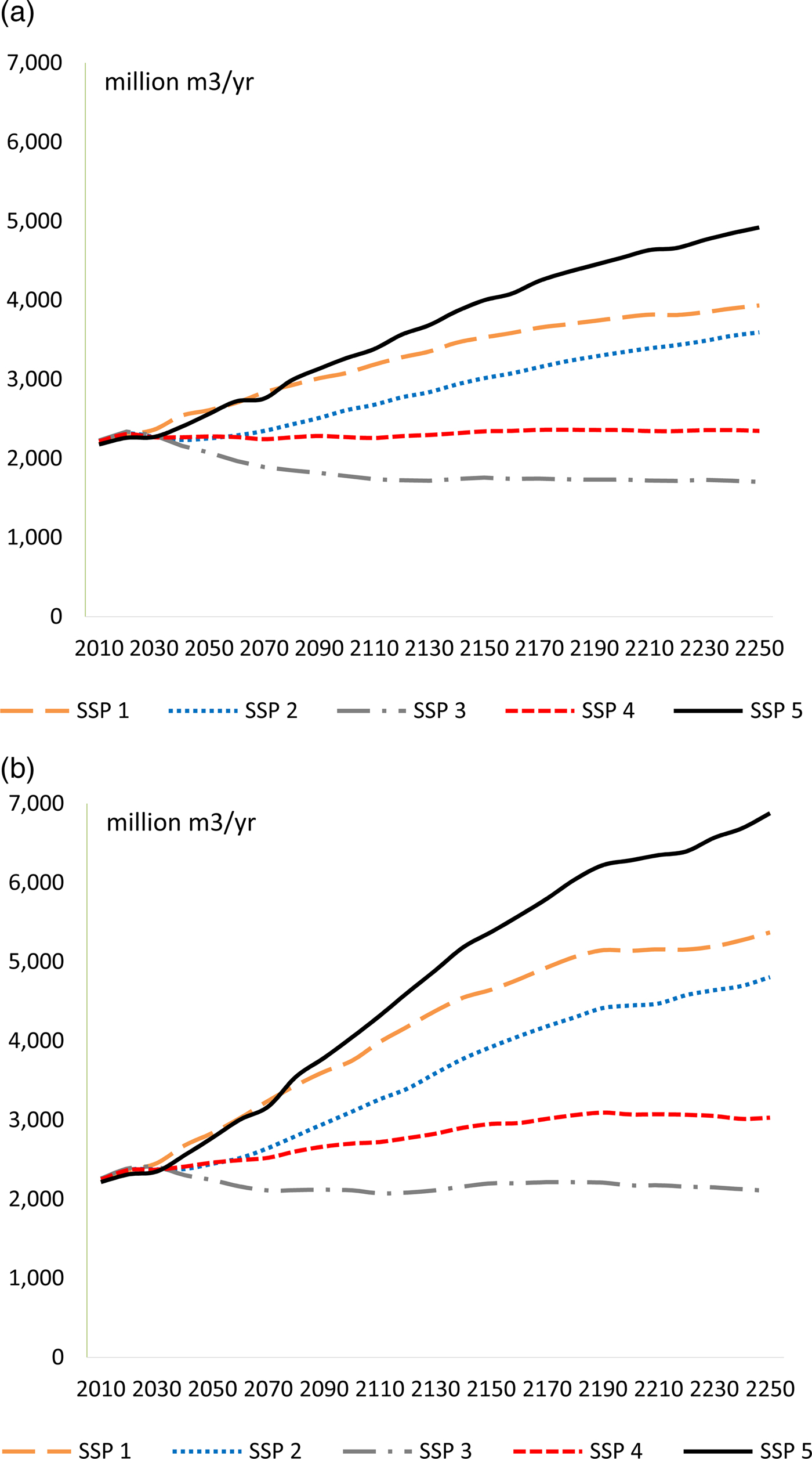
Figure 2. Global timber harvested in (a) the Baseline scenario and (b) the RCP 8.5 Scenario.
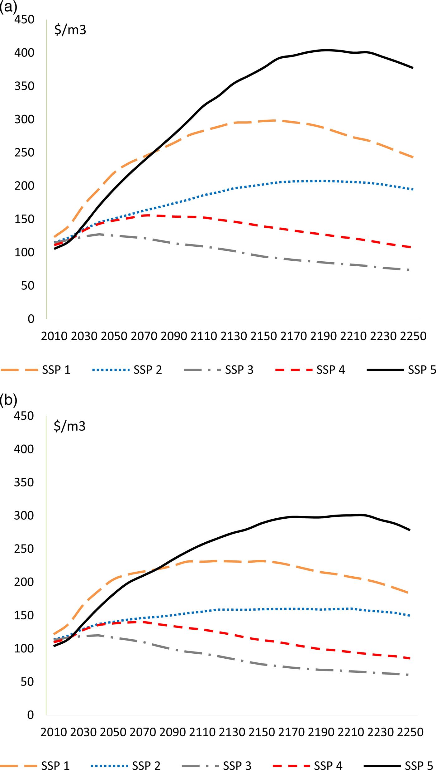
Figure 3. International price of wood in (a) the Baseline scenario and (b) the RCP 8.5 Scenario.
Global net surplus is expected to increase in all socioeconomic scenarios under the RCP 8.5, ranging from $232 billion under the SSP 3 scenario to $512 billion in the SSP 5 scenario (Table 5). Benefits accrue mostly to consumers because of the lower prices. Climate change would be mildly beneficial to producers in high latitude regions because the productivity gains outweigh the lower prices and the potential losses in stock in most cases. For instance, the yield/ha of tropical forests increases by 13–14 percent but the yield/ha of boreal and temperate forests increases by 53–78 percent depending on the socioeconomic scenario. The replacement of boreal forests by temperate forests and carbon fertilization caused a great deal of this increased productivity in high latitudes. In mid-latitudes, the timber model intensified management. Under the RCP 8.5, temperate and boreal forest regions increase their average annual timber supply for 2010–2250 by 23–40 percent while tropical regions increase their supply by only 7–8 percent relative to the Baseline.
Table 5. Present value of Regional Welfare effects under five SSP scenarios (USD Billions, r = 5%)

Note that producer surplus depends on the regional stock of forest, forest productivity, and the costs of producing timber and holding timberland. Consumer surplus, in contrast, follows timber demand that depends upon where people are located and where incomes are high enough to buy timber. The regions that enjoy the benefits of lower timber prices are not necessarily the regions with the highest forest production. The United States, Europe, and the Asian Pacific (including China) get most of the benefits from higher global timber production.
Conclusions
It is well known that the forestry sector is sensitive to climate change, but most studies have examined impacts through 2100 (e.g., Joyce et al. Reference Joyce, Mills, Heath, David McGuire, Haynes and Birdsey1995; Sohngen and Mendelsohn Reference Sohngen and Mendelsohn1998; Sohngen, Mendelsohn, and Sedjo Reference Sohngen, Mendelsohn and Sedjo2001; Perez-Garcia et al. Reference Perez-Garcia, Joyce, David McGuire and Xiao2002; Hanewinkel et al. Reference Hanewinkel, Cullmann, Schelhaas, Nabuurs and Zimmermann2013; Tian et al. Reference Tian, Sohngen, Kim, Ohrel and Cole2016) and so they have only looked at temperature changes up to 4 °C. Within this timeframe and level of warming, global forests are projected to generally expand and become more productive, increasing the net surplus in timber markets.
This is the first timber analysis to consider possible climate change impacts out to 2250. By extending the analysis to 2250, using the rapid emission scenario of RCP 8.5 and the climate model HadGEM2, this study explores the impacts of a severe climate scenario reaching 11 °C. Combining the dynamic ecosystem response of LPX-Bern DGVM with the forward-thinking dynamic global timber model (GTM), we compare a Baseline no-climate-change scenario with the RCP 8.5 outcome. The study explores long-run adjustments of forests that may occur well beyond 2100 and have been not included in other analysis. In addition, by focusing on the RCP 8.5, the analysis considers possible “catastrophic” ecosystem outcomes. Although the RCP 8.5 scenario may not be a likely outcome for the future, the scenario allows us to explore what would happen if such an extreme scenario came to pass.
The results show that forest ecosystems will be significantly affected by climate change due to changes in forest productivity and biome spatial distribution in the long run. Warming through 2190 appears to be beneficial, shifting timber supply and lowering timber prices with respect to the Baseline. The ecosystem model projects big productivity gains from biome shifts towards more productive species and from carbon fertilization. These productivity effects dwarf the loss of forestland as some forests become savannah, parkland, and woodlands. Climate change causes an increase in global timber supply through 2190 as temperatures reach 8 °C. Beyond this point, however, productivity increases shrink as carbon concentrations stabilize and temperature damage increases. Additional warming continues to shrink forestland and biomass.
Outside the timber market, the RCP 8.5 reduces global forestland by 30 percent and natural forestland by 34–38 percent with respect to the Baseline by 2250. The largest losses are in boreal forest, which almost disappears. Some of this boreal forest becomes temperate forest. But, Russia loses approximately 580 Mha of forestland. A great deal of this lost forest is natural forestland. The global forest sector will survive an 11 °C warming, but one cost of rapid warming is the loss of vast natural forestland of about 750 Mha. Most of this decline will occur in the 22nd century, when the increase in warming is the greatest.
There remain some important topics to study in this field. This study presents one extreme outcome, focusing only on the RCP 8.5 future climate projection from the climate model HadGEM2. Future research will explore more emission scenarios and other climate-model scenarios.
Second, this study finds that biomass falls in the RCP 8.5 scenario. This has huge implications for storing carbon in forests. This study did not explore carbon sequestration policies or efforts to use forests for bioenergy (Favero, Mendelsohn, and Sohngen Reference Favero, Mendelsohn and Sohngen2017). But analyses of these mitigation strategies in the context of extensive warming is clearly an important topic for future research.
Third, the DGVM and the GTM do not examine how future climate and other forces might change agriculture. In general, the study found that climate change led the forest sector to intensify production allowing it to use less land. But a future world with extensive warming may need ever more land for agriculture. An exploration of the implications of extensive warming on land use is another useful extension.
Finally, the modeling suggests that there will be an extensive loss of natural forestland in a rapid warming scenario. This has huge implications for conservation policies to protect habitat and wildlife species as well as carbon sequestration. It may also have large implications for recreation and tourism.
Appendix 1
Table A1. Summary of studies on climate change impacts on forests


 Open access