


Nomenclature
- $\textrm{DNN}$
-
deep neural network
-
$\textrm{DNN-RPM}$
-
DNN-based rapid planning method
-
$\textrm{ECI}$
-
Earth-centred inertial frame
-
$\textrm{LVLH}$
-
local vertical/local horizontal
-
$\textrm{MFT}$
-
minimum flight time
-
$\textrm{MSE}$
-
mean square error
-
$\textrm{NMC}$
-
natural-motion circumnavigation
-
$\textrm{SCP}$
-
sequential convex programming
-
$\textrm{SDP}$
-
semidefinite programmes
-
$\textrm{SQP}$
-
sequential quadratic programming
-
$b$
-
semi-minor axis of in-plane ellipse of NMC orbit (m)
-
$c$
-
maximum displacement of NMC orbit in z-axis (m)
-
$g_0$
-
gravitational acceleration at sea level (m/s2)
-
$I_{sp}$
-
vacuum specific impulse of thruster (s)
-
$J_1$
-
performance metric of Problem 1
-
$J_2$
-
performance metric of Problem 2
-
$J_3$
-
performance metric of root-finding problem
-
${\bar J_3}$
-
preset boundary value of J 3
-
$m$
-
mass of deputy spacecraft (kg)
-
$m_{\textrm{0}}$
-
initial mass deputy spacecraft (kg)
-
$M$
-
maximum iteration of hybrid search method
-
$p, p^{\prime}$
-
initial parameter and normalised parameter
-
$p_{\textrm{min}}, p_{\textrm{max}}$
-
minimum and maximum values of initial parameter
-
$\boldsymbol{r}$
-
relative position of deputy spacecraft (m)
-
$\boldsymbol{r}_c$
-
position vector of chief spacecraft (m)
-
$\boldsymbol{r}_{d}$
-
position vector of deputy spacecraft (m)
-
$t_f$
-
terminal flight time (s)
-
$t_f^*$
-
minimum flight time (s)
-
$t_{\textrm{LB}}, t_{\textrm{UB}}$
-
upper limit and lower limit of flight time (s)
-
$\boldsymbol{T}$
-
thrust of deputy spacecraft (N)
-
$\boldsymbol{T}^*$
-
optimal thrust of time-optimal control problem
-
$T_{\textrm{max}}$
-
maximum thrust (N)
-
$u$
-
adjusting parameter of thrust magnitude
-
$\boldsymbol{v}$
-
relative velocity of deputy spacecraft (m/s)
-
$\boldsymbol{x}$
-
relative state of deputy spacecraft (m, m/s)
-
$\boldsymbol{x}_{\textrm{0}}, \boldsymbol{x}_f$
-
initial and terminal relative states of deputy spacecraft (m, m/s)
-
$y_{\textrm{c}}$
-
displacement of in-plane ellipse centre in y-axis (m)
-
${y_i}$
,
${\hat y_i}$
-
real value and predicted value of DNN
-
$\varepsilon$
-
tolerance value of hybrid search method
-
$\boldsymbol{\varepsilon}$
-
angular acceleration of chief spacecraft (rad/s2)
-
$\boldsymbol{\omega}$
-
angular velocity of chief spacecraft (rad/s)
-
$\mu $
-
gravitational constant of Earth (m3/s2)
-
$\boldsymbol{\theta}$
-
unit direction vector of thrust
-
$\boldsymbol{H}$
-
Hamiltonian function
-
$\boldsymbol{\lambda }$
-
costate of states variables
-
${\boldsymbol{\lambda}_r}$
-
costate of position variables
-
${\boldsymbol{\lambda}_v}$
-
costate of velocity variables
-
${\lambda _m}$
-
costate of mass
-
$\phi $
-
phase angle of the in-plane motion (rad)
-
$\boldsymbol{\phi} $
-
performance index of time-optimal control problem
-
$\psi $
-
phase angle of the out-plane motion (rad)
-
$\boldsymbol{\psi}$
-
terminal boundary conditions
-
$\boldsymbol{\upsilon}$
-
Lagrangian multiplier vector
-
$\rho $
-
switching function


1.0 Introduction
The time-optimal trajectory planning aims at finding the time histories of the spacecraft’s position and velocity, while minimising the flight time and observing the various boundary and path constraints [Reference Zhuang and Huang1]. The limited onboard computing resources make trajectory autonomous planning challenging, especially in multi-satellites manoeuver scenarios, thus it’s urgent to develop rapid planning methods for time-optimal rendezvous problem.
Trajectory planning for spacecraft rendezvous is one of the enabling technologies for various space missions, such as rendezvous and docking [Reference Leomanni, Quartullo, Bianchini, Garulli and Giannitrapani2, Reference Jewison and Miller3], on-orbit servicing [Reference Boge and Benninghoff4], and swarm reconfiguration [Reference Bandyopadhyay, Foust, Subramanian and Hadaegh5, Reference Scala, Gaias, Colombo and Martín6]. Extensive work has been conducted on fuel/energy optimal trajectory planning by different strategies that can be mainly classified into two categories, the direct and indirect methods [Reference Betts7]. Due to the complicated nonlinear dynamics, the construction of first-order necessary conditions of optimality usually becomes costly, limiting the further application of the indirect method [Reference Morgan, Chung and Hadaegh8]. Direct methods parameterise control space (sometimes the state space) and reduce the optimal control problem to nonlinear programming problem [Reference Chai9], mainly including pseudo-spectral method [Reference Wu, Wang, Poh and Xu10, Reference Li11], mixed integer linear programming [Reference Mauro, Spiller, Bevilacqua and Curti12], and symplectic algorithms [Reference Cheng, Wen and Jin13, Reference Peng and Jiang14]. Although effective results were achieved, most of the previous studies suffered from computational efficiency due to the increasing number of spacecraft. Recently, the convex optimisation algorithm has been found to be a promising technique for online planning since its superior advantages on computational efficiency. Researchers have applied the convex optimisation and its derived sequential convex programming (SCP) in three-body problem [Reference Kayama, Howell, Bando and Hokamoto15], hypersonic vehicle reentry [Reference Xie, He, Zhang and Tang16] and interplanetary transfer [Reference Morelli, Hofmann and Topputo17], Han’s research shows that the SCP has higher computational efficiency in comparison with the pseudo-spectral method [Reference Han, Qiao, Chen and Li18]. In addition, the convex algorithm can be written using available CVX toolbox, and the resulting semidefinite programmes (SDP) would then be solved by mature solvers, such as SDPT3 and SeDuMi [Reference Grant and Boyd19]. Unfortunately, the objective function of time-optimal control problem is non-convex, which is intractable for convex optimisation algorithm. Yang innovatively used the minimum landing error problem as a gateway to solving the time-optimal asteroid landing problem, and searched for the minimum flight time (MFT) through a combination of extrapolation and bisection methods [Reference Yang, Bai and Baoyin20]. However, the performance of interpolation depends on the quality of initial guess, and iteration steps will increase with poor start points. In addition, the calculation time increases dramatically with the swarm size when it comes to satellite swarm.
With the rapid development of artificial intelligence technology, more and more scholars have combined the emerging neural network technologies with the traditional numerical optimisation methods to solve the trajectory planning problems [Reference Cheng, Li, Wang and Jiang21]. Viavattene [Reference Viavattene and Ceriotti22] applied artificial neural networks to quickly predict the time and fuel consumption of interplanetary low-thrust transfers, and the predicted result was used to search the feasible asteroid rendezvous sequence. Considering the reentry trajectory planning of hypersonic vehicles, Wang [Reference Wang, Wu, Liu, Yang and Liang23] utilised the Chebyshev pseudo-spectral method to generate optimal trajectory dataset and established a neural network to predict the control variables. In Ref. [Reference Dai, Feng, Feng, Cui and Zhang24], the sequential second-order cone programming method was applied to generate optimal entry trajectories offline, and a neural network was trained to output the predicted control command online. However, there are inevitable errors between predicted results of neural network and optimal control commands. When it comes to the rendezvous problem, the control errors would invalidate terminal constraints, which may lead to collisions between spacecraft.
Concentrating on the time-optimal rendezvous problem, a rapid trajectory planning method based on convex optimisation and deep neural network (DNN) is proposed, which can not only improve the computational efficiency of time-optimal trajectory, but also perform well in natural-motion circumnavigation (NMC) orbit injection and swarm reconfiguration. The first contribution of this paper lies in transforming the time-optimal rendezvous problem into a double-layer optimisation framework, where the inner layer is a convex optimisation problem, and the outer layer is a root-finding problem. Inspired by the concept of minimum landing error problem in Mars and asteroid landing [Reference Yang, Bai and Baoyin20, Reference Blackmore, Açikmeşe and Scharf25], the inner layer constructs a minimum terminal error problem that takes the terminal error between the actual and desired state as optimisation index. The thrust properties corresponding to time-optimal control are analysed theoretically. The objective function of the outer root-finding problem is constructed based on the thrust magnitude and the terminal error, so that the corresponding control law is time-optimal when the objective equals zero.
The second contribution lies in proposing a hybrid search algorithm (HSM) and a deep neural network based rapid planning method (DNN-RPM) to search for MFT. For the outer layer root-finding problem, the bisection and Newton’s methods are two typical and effective iterative-based algorithms. The bisection method is robust but computationally inefficiently. The convergence rate for classical Newton’s method is at least quadratic, but it fails to converge when the Hessian matrix is not positive definite [Reference Press, Teukolsky, Vetterling and Flannery26]. In order to balance computational efficiency and robustness, the HSM that combines the advantages of above two methods is proposed to generate dataset for DNN training. And then, the DNN-RPM is put forward to further improve computational efficiency, in which the trained DNN provides a high-quality initial guess for Newton’s method. In addition, the DNN-RPM can also be used to calculate the best entering angle of NMC orbit injection problem and the minimum reconfiguration time of spacecraft swarm.
The remainder of this paper is organised as follows. Firstly, the time-optimal problem is formulated, and the optimal control is derived based on Pontryagin’s maximum principle. Then, the non-convex time-optimal problem is reformulated into a double-layer optimisation framework, making it more tractable to solve with convex programming. Thirdly, the HSM and DNN- RPM are put forward to search for MFT. Finally, comparative numerical simulations are carried out to validate the performance of the proposed optimisation framework and methods.
2.0 Problem formulation
The spacecraft rendezvous contains deputy and chief satellites, generally described in the local vertical/local horizontal (LVLH) coordinate frame attached to the mass centre of chief spacecraft. As shown in Fig. 1, r d and r c represent the position vector of deputy and chief spacecraft in the Earth centred inertial frame (ECI). The x-axis coincides with r c , the z-axis is aligned with moment of momentum, and the y-axis completes the right-hand system [Reference Zhang, Cai, Yang and Si27].
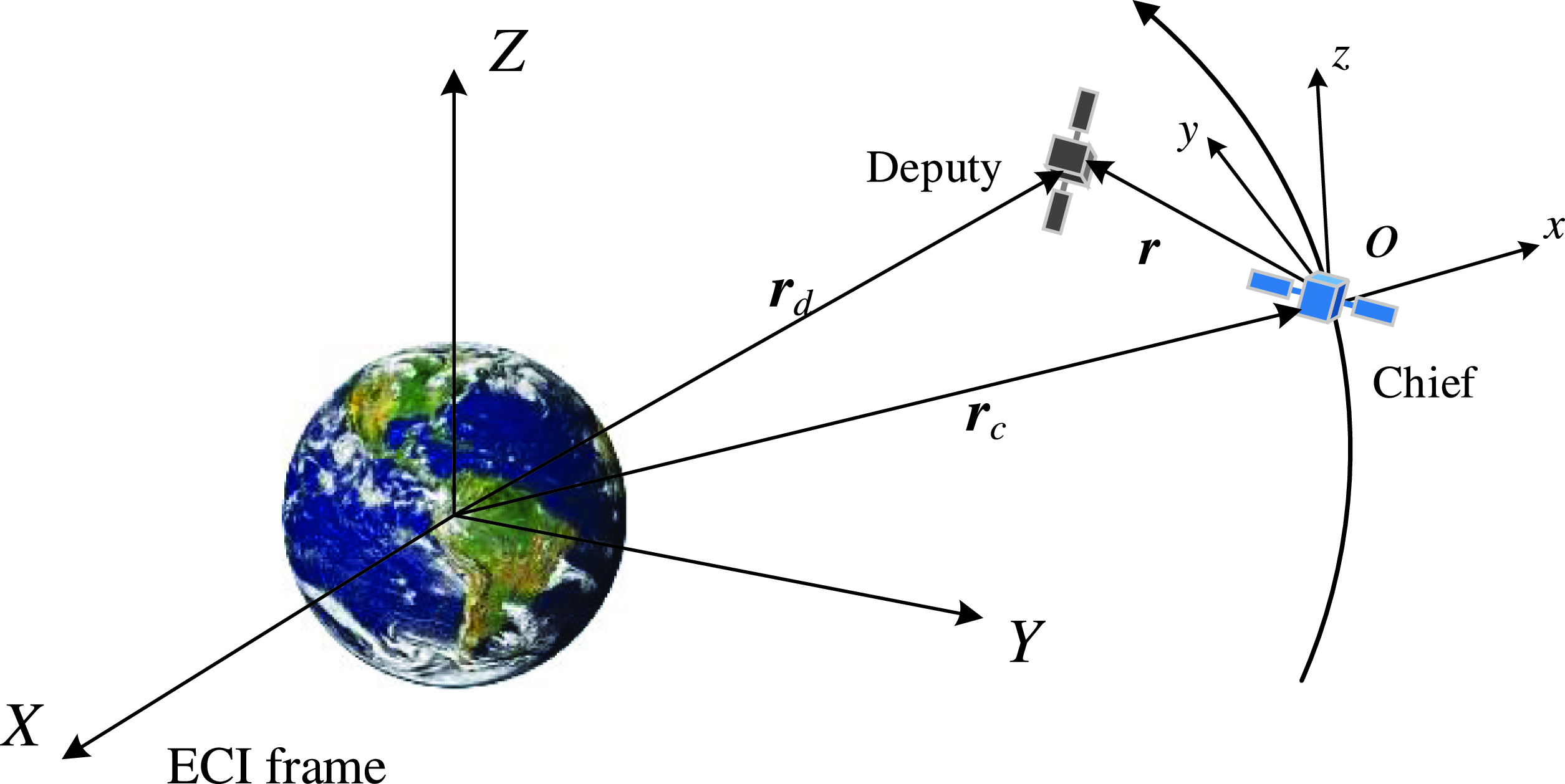
Figure 1. The description of coordinate frames.
The relative dynamic of deputy satellite in LVLH frame can be described as
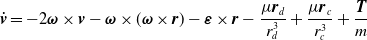 \begin{align}{\dot{\boldsymbol{v}}} = - 2\boldsymbol{\omega } \times \boldsymbol{v} - \boldsymbol{\omega } \times (\boldsymbol{\omega } \times \boldsymbol{r}) - \boldsymbol{\varepsilon } \times \boldsymbol{r} - \frac{\mu \boldsymbol{r}_d}{r_d^3} + \frac{\mu \boldsymbol{r}_c}{r_c^3} + \frac{\boldsymbol{T}}{m}\end{align}
where
r
and
v
are the relative position and velocity of deputy spacecraft,
ω
and
ε
denote the instantaneous angular velocity and acceleration of chief spacecraft,
T
and m mean the thrust and mass of deputy spacecraft, $\mu $
is the gravitational constant of Earth,
$\mu $
is the gravitational constant of Earth, ${r_d} = {\left\| {{{\boldsymbol{r}}_d}} \right\|_2}$
,
${r_d} = {\left\| {{{\boldsymbol{r}}_d}} \right\|_2}$
, ${r_c} = {\left\| {{{\boldsymbol{r}}_c}} \right\|_2}$
. If the target orbit is a near-circular orbit and its radius is much larger than relative distance simultaneously, the equation (1) can be simplified as
${r_c} = {\left\| {{{\boldsymbol{r}}_c}} \right\|_2}$
. If the target orbit is a near-circular orbit and its radius is much larger than relative distance simultaneously, the equation (1) can be simplified as
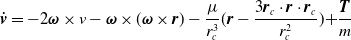 \begin{align}{\dot{\boldsymbol{v}}}= - 2\boldsymbol{\omega } \times {v} - \boldsymbol{\omega } \times (\boldsymbol{\omega } \times {\boldsymbol{r}}) - \frac{\mu }{{r_c^3}}(\boldsymbol{r} - \frac{{3{\boldsymbol{r}_c} \cdot \boldsymbol{r} \cdot {\boldsymbol{r}_c}}}{{r_c^2}}){ + }\frac{\boldsymbol{T}}{m}\end{align}
Mass consumption obeys
 \begin{align}{\dot{\boldsymbol{m}}} = - \frac{{\left\| \boldsymbol{T} \right\|}_2}{{I_{sp}}{g_0}}\end{align}
where I sp is vacuum specific impulse of thruster, g 0=9.80665m/s2 denote gravitational acceleration at sea level.
In addition, the manoeuver procedure for spacecraft rendezvous needs to satisfy boundary conditions in equation (4) and (5), and the limitation on thrust in equation (6).
 \begin{align} \boldsymbol{x}(\boldsymbol{t}_0)= \boldsymbol{x}_0,\quad \boldsymbol{m}(\boldsymbol{t}_0)=\boldsymbol{m}_0 \end{align}
 \begin{align} \boldsymbol{x}({t_f}) = {\boldsymbol{x}_f}\end{align}
 \begin{align} {\left\| \boldsymbol{T} \right\|_2} \le {T_{\max }}\end{align}
where $\boldsymbol{x}$
is the relative state of deputy spacecraft,
$\boldsymbol{x}$
is the relative state of deputy spacecraft, ${\boldsymbol{x}_0}$
and
${\boldsymbol{x}_0}$
and ${\boldsymbol{x}_f}$
are the initial and terminal relative states,
${\boldsymbol{x}_f}$
are the initial and terminal relative states, ${m_0}$
is the initial mass,
${m_0}$
is the initial mass, ${t_f}$
means terminal flight time,
${t_f}$
means terminal flight time, ${T_{\max }}$
is the maximum thrust. The time-optimal control problem can be summarised as Problem 1.
${T_{\max }}$
is the maximum thrust. The time-optimal control problem can be summarised as Problem 1.
Problem 1 (time-optimal control problem)
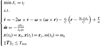 \begin{align}\left\{ \begin{array}{l}\min {J_1} = {t_f} \\[4pt] s.t.\\[4pt] {\dot{\boldsymbol{v}}} = - 2\boldsymbol{\omega } \times \boldsymbol{v} - \boldsymbol{\omega } \times (\boldsymbol{\omega } \times \boldsymbol{r}) - \frac{\mu }{{r_c^3}}\left(\boldsymbol{r} - \frac{{3{\boldsymbol{r}_c} \cdot \boldsymbol{r} \cdot {\boldsymbol{r}_c}}}{{r_c^2}}\right) + \frac{\boldsymbol{T}}{m}\\[4pt] {\dot{\boldsymbol{m}}} = - \frac{{{{\left\| \boldsymbol{T} \right\|}_2}}}{{{I_{sp}}{g_0}}}\\[4pt] \boldsymbol{x}({t_0}) = {\boldsymbol{x}_0}, \boldsymbol{x}({t_f}) = {\boldsymbol{x}_f}, m({t_0}) = {m_0}\\[4pt] {\left\| \boldsymbol{T} \right\|_2} \le {T_{\max }}\end{array} \right.\end{align}
Assumption 1. The maximum acceleration is larger than the resultant acceleration of gravitational, centripetal and Coriolis accelerations.
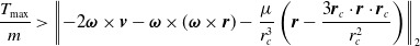 \begin{align}\frac{T_{\max }}{m} \gt {\left\| - 2\boldsymbol{\omega } \times {\boldsymbol{v}} - \boldsymbol{\omega } \times (\boldsymbol{\omega } \times {\boldsymbol{r}}) - \frac{\mu }{r_c^3}\left(\boldsymbol{r} - \frac{{3{\boldsymbol{r}_c} \cdot \boldsymbol{r} \cdot {\boldsymbol{r}_c}}}{{r_c^2}}\right) \right\|}_2\end{align}
The resultant acceleration varies with orbit height and relative states
x
and it’s of the order of ${10^{ - 5}} \sim {10^{ - 3}}{\textrm{m/}}{{\textrm{s}}^{\textrm{2}}}$
. Assumption 1 is rational and easy to satisfy since the thruster acceleration is generally greater than the relevant acceleration terms on the right-hand side.
${10^{ - 5}} \sim {10^{ - 3}}{\textrm{m/}}{{\textrm{s}}^{\textrm{2}}}$
. Assumption 1 is rational and easy to satisfy since the thruster acceleration is generally greater than the relevant acceleration terms on the right-hand side.
Proposition 1. The optimal control of Problem 1 must be ${\left\| {{\boldsymbol{T}^*}} \right\|_2}\, = \,{T_{\max }}$
when
${\left\| {{\boldsymbol{T}^*}} \right\|_2}\, = \,{T_{\max }}$
when $t \lt {t_f}$
, and
$t \lt {t_f}$
, and ${\left\| {{\boldsymbol{T}^*}} \right\|_2} \le {T_{\max }}$
can only happen at t=t
f
and
${\left\| {{\boldsymbol{T}^*}} \right\|_2} \le {T_{\max }}$
can only happen at t=t
f
and ${\boldsymbol{\lambda }_{v}}({t_f}) = 0$
.
${\boldsymbol{\lambda }_{v}}({t_f}) = 0$
.
Proof. Denoting the thrust as
 \begin{align}\boldsymbol{T} = {T_{\max }}u\boldsymbol{\theta }\end{align}
where $u \in [0,1]$
is the parameter to adjust thrust magnitude,
$u \in [0,1]$
is the parameter to adjust thrust magnitude, $\boldsymbol{\theta}$
denotes the unit direction vector.
$\boldsymbol{\theta}$
denotes the unit direction vector.
Assuming that the $t_f^*$
and
$t_f^*$
and ${\boldsymbol{T}^*}$
are the MFT and optimal control for Problem 1. According to Pontryagin’s maximum principle, the Hamiltonian function for Problem 1 is
${\boldsymbol{T}^*}$
are the MFT and optimal control for Problem 1. According to Pontryagin’s maximum principle, the Hamiltonian function for Problem 1 is
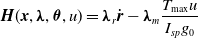
 \begin{align}\boldsymbol{H}(\boldsymbol{x},\boldsymbol{\lambda },\boldsymbol{\theta },u) = \boldsymbol{\lambda }_r\dot{\boldsymbol{r}} + \boldsymbol{\lambda }_v\left[ - 2\boldsymbol{\omega } \times {\boldsymbol{v}- \boldsymbol{\omega} } \times (\boldsymbol{\omega } \times r) - \frac{\mu }{{r_2^3}}(\boldsymbol{r} - \frac{{3{\boldsymbol{r}_2} \cdot \boldsymbol{r} \cdot {\boldsymbol{r}_2}}}{{r_2^2}}) + \frac{{{T_{\max }}u\boldsymbol{\theta }}}{m}\right] - {\boldsymbol{\lambda }_m}\frac{{{T_{\max }}u}}{{{I_{sp}}{g_0}}}\end{align}
The costates $\boldsymbol{\lambda } = {[{\lambda _x},{\lambda _y},{\lambda _z},{\lambda _{{v_x}}},{\lambda _{{v_y}}},{\lambda _{{v_z}}},{\lambda _m}]^{\textrm{T}}}$
satisfy the following differential equations and transversality condition,
$\boldsymbol{\lambda } = {[{\lambda _x},{\lambda _y},{\lambda _z},{\lambda _{{v_x}}},{\lambda _{{v_y}}},{\lambda _{{v_z}}},{\lambda _m}]^{\textrm{T}}}$
satisfy the following differential equations and transversality condition,
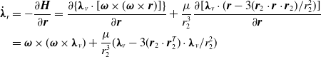 \begin{align}{{\boldsymbol{\dot \lambda }}_r} &= - \frac{{\partial \boldsymbol{H}}}{{\partial \boldsymbol{r}}} = \frac{\partial \{ {\boldsymbol{\lambda }_v} \cdot [\boldsymbol{\omega } \times (\boldsymbol{\omega } \times \boldsymbol{r})]\} }{\partial \boldsymbol{r}} + \frac{\mu }{r_2^3}\frac{\partial [{\boldsymbol{\lambda }_v} \cdot (\boldsymbol{r} - 3({\boldsymbol{r}_2} \cdot \boldsymbol{r} \cdot {\boldsymbol{r}_2}) / {r_2^2})]}{\partial \boldsymbol{r}}\nonumber\\ &= \boldsymbol{\omega } \times (\boldsymbol{\omega } \times {\boldsymbol{\lambda }_v}) + \frac{\mu }{r_2^3}({\boldsymbol{\lambda}_v}-3(\boldsymbol{r}_2 \cdot \boldsymbol{r}_2^T) \cdot \boldsymbol{\lambda }_v / {r_2^2})\end{align}
 \begin{align}\boldsymbol{\dot \lambda }_v = - \frac{\partial \boldsymbol{H}}{{\partial {\boldsymbol{v}}}} = - {\boldsymbol{\lambda }_r} + 2\frac{{\partial [{\boldsymbol{\lambda }_v} \cdot (\boldsymbol{\omega } \times {v})]}}{{\partial {\boldsymbol{H}}}} = - {\boldsymbol{\lambda }_r} + 2{\boldsymbol{\lambda }_v} \times \boldsymbol{\omega }\end{align}
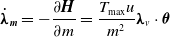 \begin{align}\dot{\boldsymbol{\lambda}}_{\boldsymbol{m}} = - \frac{{\partial \boldsymbol{H}}}{{\partial m}} = \frac{{{T_{\max }}u}}{{{m^2}}}{\boldsymbol{\lambda }_v} \cdot \boldsymbol{\theta }\end{align}
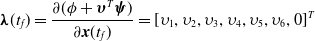 \begin{align}\boldsymbol{\lambda }({t_f}) = \frac{{\partial (\phi + {\boldsymbol{\upsilon}^T}\boldsymbol{\psi})}}{{\partial \boldsymbol{x}({t_f})}} = {[{\upsilon _1},{\upsilon _2},{\upsilon _3},{\upsilon _4},{\upsilon _5},{\upsilon _6},0]^T}\end{align}
where ${\boldsymbol{\lambda }_r} = {[{\lambda _x},{\lambda _y},{\lambda _z}]^{\textrm{T}}}$
,
${\boldsymbol{\lambda }_r} = {[{\lambda _x},{\lambda _y},{\lambda _z}]^{\textrm{T}}}$
, ${\boldsymbol{\lambda }_r} = {[{\lambda _{{v_x}}},{\lambda _{{v_y}}},{\lambda _{{v_z}}}]^{\textrm{T}}}$
,
${\boldsymbol{\lambda }_r} = {[{\lambda _{{v_x}}},{\lambda _{{v_y}}},{\lambda _{{v_z}}}]^{\textrm{T}}}$
, $\phi $
and
$\phi $
and ${\psi }$
are the performance index and terminal boundary conditions, respectively.
${\psi }$
are the performance index and terminal boundary conditions, respectively. ${\upsilon }$
is the Lagrangian multiplier vector. Since there is no boundary condition for m at t
f
,
${\upsilon }$
is the Lagrangian multiplier vector. Since there is no boundary condition for m at t
f
, ${\lambda _m}({t_f}) = 0$
.
${\lambda _m}({t_f}) = 0$
.
The optimal terminal condition is
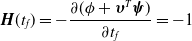 \begin{align}\boldsymbol{H}({t_f}) = - \frac{{\partial (\phi + {\boldsymbol{\upsilon }^T}\boldsymbol{\psi })}}{{\partial {t_f}}} = - 1\end{align}
Case 1: $\left\| {{\boldsymbol{\lambda }_v}} \right\| \ne 0$
at
$\left\| {{\boldsymbol{\lambda }_v}} \right\| \ne 0$
at $t \in [{t_0},{t_f}]$
.
$t \in [{t_0},{t_f}]$
.
The optimal control is used to minimise Hamiltonian function,
 \begin{align}\min \boldsymbol{H}({\boldsymbol{x}^ * },{\boldsymbol{\lambda }^ * },\boldsymbol{\theta },u) = \boldsymbol{H}({\boldsymbol{x}^ * },{\boldsymbol{\lambda }^ * },{\boldsymbol{\theta }^ * },{u^ * })\end{align}
Hence the optimal direction and magnitude of optimal control are
 \begin{align}{\boldsymbol{\theta }^*} = - \frac{{{\boldsymbol{\lambda }_v}}}{{\left\| {{\boldsymbol{\lambda }_v}} \right\|}}\end{align}
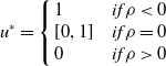 \begin{align}{u^*} = \left\{ \begin{array}{l@{\quad}l}1 & {if \rho \lt 0}\\ \left[0,1\right] & {if \rho = 0}\\ 0 &{if \rho \gt 0}\end{array}\right.\end{align}
The switching function $\rho $
is
$\rho $
is
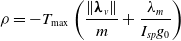 \begin{align}\rho = - {T_{\max }}\left(\frac{{\left\| {{\boldsymbol{\lambda }_v}} \right\|}}{m} + \frac{{{\lambda _m}}}{{{I_{sp}}{g_0}}}\right)\end{align}
Since ${\lambda _m}({t_f}) = 0$
and
${\lambda _m}({t_f}) = 0$
and ${\dot \lambda _m} \lt 0$
, thus
${\dot \lambda _m} \lt 0$
, thus
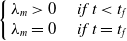 \begin{align}\left\{ \begin{array}{cc}\lambda _m \gt 0 &\quad {if\, t \lt {t_f}}\\ {\lambda _m} = 0 &\quad {if\, t = {t_f}}\end{array} \right.\end{align}
Substituting equation (20) into (19), the switching function $\rho \lt 0$
. Therefore, if
$\rho \lt 0$
. Therefore, if ${\boldsymbol{\lambda }_v} \ne 0$
at
${\boldsymbol{\lambda }_v} \ne 0$
at $t \in [{t_0},{t_f}]$
,
$t \in [{t_0},{t_f}]$
, ${u^*} = 1$
, namely
${u^*} = 1$
, namely ${\left\| {{\boldsymbol{T}^*}} \right\|_2}\, = \,{T_{\max }}$
.
${\left\| {{\boldsymbol{T}^*}} \right\|_2}\, = \,{T_{\max }}$
.
Case 2: ${\boldsymbol{\lambda }_v} = 0$
occurs in one or more time intervals.
${\boldsymbol{\lambda }_v} = 0$
occurs in one or more time intervals.
Assuming that ${\boldsymbol{\lambda }_v} = 0$
at
${\boldsymbol{\lambda }_v} = 0$
at $t \in [{t_i},{t_j}]$
, so
$t \in [{t_i},{t_j}]$
, so ${{\dot \lambda }_v}$
is zero,
${{\dot \lambda }_v}$
is zero, ${\dot \lambda _m} = {{\dot \lambda }_r}\, = \,{\boldsymbol{\lambda }_r}\, = \,0$
can then be derived according to equations (11)–(13);. Since
${\dot \lambda _m} = {{\dot \lambda }_r}\, = \,{\boldsymbol{\lambda }_r}\, = \,0$
can then be derived according to equations (11)–(13);. Since ${\boldsymbol{\lambda }_r} = {{\dot \lambda }_r} = 0$
at
${\boldsymbol{\lambda }_r} = {{\dot \lambda }_r} = 0$
at $t \in [{t_i},{t_j}]$
,
$t \in [{t_i},{t_j}]$
, ${\boldsymbol{\lambda }_r}$
will stay at zero when
${\boldsymbol{\lambda }_r}$
will stay at zero when $t \in [{t_j},{t_f}]$
. In the same way,
$t \in [{t_j},{t_f}]$
. In the same way, ${\boldsymbol{\lambda }_v}$
stay at zero when
${\boldsymbol{\lambda }_v}$
stay at zero when $t \in [{t_j},{t_f}]$
.
$t \in [{t_j},{t_f}]$
.
According to equation (10), $\boldsymbol{H}({t_f}) = 0$
since
$\boldsymbol{H}({t_f}) = 0$
since ${\boldsymbol{\lambda }_r}({t_f}) = {\boldsymbol{\lambda }_v}({t_f}) = {\lambda _m}({t_f}) = 0$
, which however contradicts to equation (15). Therefore, the assumption is invalid, and case 2 will not happen.
${\boldsymbol{\lambda }_r}({t_f}) = {\boldsymbol{\lambda }_v}({t_f}) = {\lambda _m}({t_f}) = 0$
, which however contradicts to equation (15). Therefore, the assumption is invalid, and case 2 will not happen.
Case 3: ${\boldsymbol{\lambda }_v} = 0$
occurs at some discrete points when
${\boldsymbol{\lambda }_v} = 0$
occurs at some discrete points when $t \in [{t_0},{t_f}]$
.
$t \in [{t_0},{t_f}]$
.
If ${\boldsymbol{\lambda }_v} = 0$
, the equation (10) can be reduced as
${\boldsymbol{\lambda }_v} = 0$
, the equation (10) can be reduced as
 \begin{align}\boldsymbol{H}(\boldsymbol{x},\boldsymbol{\lambda },\boldsymbol{\theta },u) = {\boldsymbol{\lambda }_r}{{\dot{\boldsymbol{r}}}} - {\boldsymbol{\lambda }_m}\frac{{{T_{\max }}u}}{{{I_{sp}}{g_0}}}\end{align}
Accordingly, $\rho $
is
$\rho $
is
 \begin{align}\rho = - \frac{{{T_{\max }}{\lambda _m}}}{{{I_{sp}}{g_0}}}\end{align}
The equations (17)–(20) still hold for all other points where $\left\| {{\boldsymbol{\lambda }_v}} \right\| \ne 0$
. Only if
$\left\| {{\boldsymbol{\lambda }_v}} \right\| \ne 0$
. Only if $t = {t_f}$
and
$t = {t_f}$
and ${\boldsymbol{\lambda }_v}({t_f}) = 0$
,
${\boldsymbol{\lambda }_v}({t_f}) = 0$
, $\rho = 0$
, so
$\rho = 0$
, so ${u^*} = [0,1]$
. Otherwise,
${u^*} = [0,1]$
. Otherwise, $\rho \lt 0$
and
$\rho \lt 0$
and ${u^*} = 1$
still hold.
${u^*} = 1$
still hold.
According to the analysis of above three cases, the magnitude of optimal thrust always remains at maximum when t<t
f
, and ${\left\| {{\boldsymbol{T}^*}} \right\|_2}\, = \,{T_{\max }}$
can only happen at t=t
f
and
${\left\| {{\boldsymbol{T}^*}} \right\|_2}\, = \,{T_{\max }}$
can only happen at t=t
f
and $\lambda ({t_f}) = 0$
.
$\lambda ({t_f}) = 0$
.
3.0 The double-layer optimisation framework
In this section, the minimum terminal error problem, which can be described as convex form, is introduced firstly, and then a double-layer optimisation framework is proposed to search for MFT. Taking the terminal error between actual and desired state as objective, the minimum terminal error problem at given flight time ${t_f}$
can be described as follows,
${t_f}$
can be described as follows,
Problem 2 (Minimum-terminal-error problem)
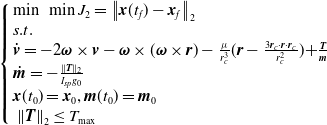 \begin{align}\left\{ \begin{array}{l}\min\,\, \min {J_2} = {\left\| {\boldsymbol{x}({t_f}) - {\boldsymbol{x}_f}} \right\|_2}\\s.t.\\{\dot{\boldsymbol{v}}} = - 2\boldsymbol{\omega } \times \boldsymbol{v} - \boldsymbol{\omega } \times (\boldsymbol{\omega } \times {\boldsymbol{r}}) - \frac{\mu }{{r_c^3}}(\boldsymbol{r} - \frac{{3{\boldsymbol{r}_c} \cdot \boldsymbol{r} \cdot {\boldsymbol{r}_c}}}{{r_c^2}}){ + }\frac{\boldsymbol{T}}{{\boldsymbol{m}}}\\{\dot{\boldsymbol{m}}} = - \frac{{{{\left\| \boldsymbol{T} \right\|}_2}}}{{{I_{sp}}{g_0}}}\\ \boldsymbol{x}({t_0}) = {\boldsymbol{x}_0} , {\boldsymbol{m}}({t_0}) = {{\boldsymbol{m}}_0}\\ \,{\left\| \boldsymbol{T} \right\|_2} \le {T_{\max }}\end{array} \right.\end{align}
It’s worth noting that the objective and inequality constraints of Problem 2 are convex functions, and equality constraints are affine form, so it could be transformed into a convex optimisation problem. There are some propositions for Problem 2.
Proposition 2. The optimal objective of Problem 2 is larger than zero when ${t_f} \lt t_f^*$
, and the optimal objective is equal to zero when
${t_f} \lt t_f^*$
, and the optimal objective is equal to zero when ${t_f} \geqslant t_f^*$
.
${t_f} \geqslant t_f^*$
.
Proof: Assuming that the optimal objective ${J_2}({t_f})\, = \,0$
when
${J_2}({t_f})\, = \,0$
when ${t_f} \lt t_f^*$
, namely
${t_f} \lt t_f^*$
, namely $\boldsymbol{x}({t_f}) - {\boldsymbol{x}_f}\, = \,0$
. It means that
$\boldsymbol{x}({t_f}) - {\boldsymbol{x}_f}\, = \,0$
. It means that ${t_f}$
is a feasible solution for Problem 1 and
${t_f}$
is a feasible solution for Problem 1 and ${t_f} \lt t_f^*$
, which however is contrary to the definition of time-optimal control problem. Therefore, the optimal objective of Problem 2 is more than zero when
${t_f} \lt t_f^*$
, which however is contrary to the definition of time-optimal control problem. Therefore, the optimal objective of Problem 2 is more than zero when ${t_f} \lt t_f^*$
.
${t_f} \lt t_f^*$
.
If ${t_f} = t_f^*$
, the optimal solution to Problem 1 is such that
${t_f} = t_f^*$
, the optimal solution to Problem 1 is such that $\boldsymbol{x}({t_f}) - {\boldsymbol{x}_f}\, = \,0$
, and hence the optimal objective of Problem 2 is zero.
$\boldsymbol{x}({t_f}) - {\boldsymbol{x}_f}\, = \,0$
, and hence the optimal objective of Problem 2 is zero.
When ${t_f} \gt t_f^*$
, the following control is feasible for Problem 2, and the objective remains zero.
${t_f} \gt t_f^*$
, the following control is feasible for Problem 2, and the objective remains zero.
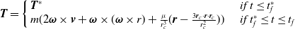 \begin{align}\boldsymbol{T} = \left\{ \begin{array}{ll}{\boldsymbol{T}^*} &\quad if\, t \le t_f^*\\ m(2\boldsymbol{\omega } \times {\boldsymbol{v}} + \boldsymbol{\omega } \times (\boldsymbol{\omega } \times r) + \frac{\mu }{{r_c^3}}(\boldsymbol{r} - \frac{{3{\boldsymbol{r}_c} \cdot \boldsymbol{r} \cdot {\boldsymbol{r}_c}}}{{r_c^2}}) ) & \quad if\, t_f^* \le t \le {t_f} \end{array} \right.\end{align}
Proposition 3. The optimal thrust of Problem 2 must be ${\left\| {{\boldsymbol{T}^*}} \right\|_2}\, = \,{T_{\max }}$
when
${\left\| {{\boldsymbol{T}^*}} \right\|_2}\, = \,{T_{\max }}$
when ${t_f} \lt t_f^*$
.
${t_f} \lt t_f^*$
.
Proof: Since the Hamiltonian function and costates function of Problem 2 are the same as Problem 1, the analysis of cases 1 and 3 still hold for Problem 2. When it comes to case 2, the transversality condition for minimum terminal error problem is
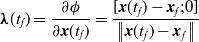 \begin{align}\boldsymbol{\lambda }({t_f}) = \frac{{\partial \phi }}{{\partial \boldsymbol{x}({t_f})}} = \frac{{[\boldsymbol{x}({t_f}) - {\boldsymbol{x}_f};0]}}{{\left\| {\boldsymbol{x}({t_f}) - {\boldsymbol{x}_f}} \right\|}}\end{align}
According to Proposition 2, $\boldsymbol{x}({t_f}) \ne {\boldsymbol{x}_f}$
when
$\boldsymbol{x}({t_f}) \ne {\boldsymbol{x}_f}$
when ${t_f} \lt t_f^*$
, thus
${t_f} \lt t_f^*$
, thus $\left\| {\boldsymbol{\lambda }({t_f})} \right\| \ne 0$
, which contradicts with the condition that
$\left\| {\boldsymbol{\lambda }({t_f})} \right\| \ne 0$
, which contradicts with the condition that $\left\| {\boldsymbol{\lambda }({t_f})} \right\| = 0$
.
$\left\| {\boldsymbol{\lambda }({t_f})} \right\| = 0$
.
Proposition 4. If ${t_f} \le t_f^*$
, the optimal terminal error for Problem 2 decreases with
${t_f} \le t_f^*$
, the optimal terminal error for Problem 2 decreases with ${t_f}$
.
${t_f}$
.
Proof: If ${t_a} \lt {t_b} \le t_f^*$
,
${t_a} \lt {t_b} \le t_f^*$
, $\boldsymbol{T}_a^* $
and
$\boldsymbol{T}_a^* $
and $\boldsymbol{T}_b^* $
are the corresponding optimal control, assuming that
$\boldsymbol{T}_b^* $
are the corresponding optimal control, assuming that ${\boldsymbol{T}_b}$
is
${\boldsymbol{T}_b}$
is
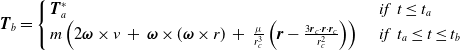 \begin{align}{\boldsymbol{T}_b} = \left\{\begin{array}{ll}\boldsymbol{T}_a^* &\quad if\,\, t \le {t_a} \\ m\left(2\boldsymbol{\omega } \times {v}\, + \,\boldsymbol{\omega } \times (\boldsymbol{\omega } \times r)\, + \,\frac{\mu }{{r_c^3}}\left(\boldsymbol{r} - \frac{{3{\boldsymbol{r}_c} \cdot \boldsymbol{r} \cdot {\boldsymbol{r}_c}}}{{r_c^2}}\right)\right) & \quad if\,\, {t_a} \le t \le {t_b}\end{array} \right.\end{align}
It’s evident that $J({\boldsymbol{T}_b}) = J(\boldsymbol{T}_a^*)$
. In addition,
$J({\boldsymbol{T}_b}) = J(\boldsymbol{T}_a^*)$
. In addition, $J({\boldsymbol{T}_b}) \lt J(\boldsymbol{T}_b^*)$
according to Proposition 3. Therefore, J(
T
b
)=
$J({\boldsymbol{T}_b}) \lt J(\boldsymbol{T}_b^*)$
according to Proposition 3. Therefore, J(
T
b
)= $J(\boldsymbol{T}_a^*) \lt J(\boldsymbol{T}_b^*)$
when
$J(\boldsymbol{T}_a^*) \lt J(\boldsymbol{T}_b^*)$
when ${t_a} \lt {t_b} \le t_f^*$
.
${t_a} \lt {t_b} \le t_f^*$
.
Based on the analysis in Propositions 2 and 4, the minimum terminal error J
2 decreases monotonically as ${t_f}$
when
${t_f}$
when ${t_f} \lt t_f^*$
and remains zero when
${t_f} \lt t_f^*$
and remains zero when ${t_f} \geqslant t_f^*$
. Therefore, the MFT is equal to the turning point where J
2=0.
${t_f} \geqslant t_f^*$
. Therefore, the MFT is equal to the turning point where J
2=0.
Unfortunately, this kind of root-finding problem is still intractable for typical search algorithms, such as the bisection and Newton’s method. As shown in Fig. 2, if the iterative points ${t_n}$
and
${t_n}$
and ${t_{n + 1}}$
are far away
${t_{n + 1}}$
are far away $t_f^*$
or once the iterative points lie on the right of
$t_f^*$
or once the iterative points lie on the right of $t_f^*$
, Newton’s method will not converge. The bisection method is also infeasible since it iterates over two values with opposite signs, while J
2 remains zero when
$t_f^*$
, Newton’s method will not converge. The bisection method is also infeasible since it iterates over two values with opposite signs, while J
2 remains zero when ${t_f} \geqslant t_f^*$
.
${t_f} \geqslant t_f^*$
.
Inspired by Proposition 3, a new performance metrics is constructed as follows
 \begin{align}{J_3} = {\left\| {x({t_f}) - {x_f}} \right\|_2} - \int_{{t_0}}^{{t_f}} {\left| {{{\left\| {{\bf\boldsymbol{T}}(t)} \right\|}_2} - {T_{\max }}} \right|} dt\end{align}
Proposition 5. ${J_3} \gt 0$
when
${J_3} \gt 0$
when ${t_f} \lt t_f^*$
,
${t_f} \lt t_f^*$
, ${J_3} = 0$
when
${J_3} = 0$
when ${t_f} = t_f^*$
, and
${t_f} = t_f^*$
, and ${J_3} \lt 0$
when
${J_3} \lt 0$
when ${t_f} \gt t_f^*$
.
${t_f} \gt t_f^*$
.
Proof: As shown in Table 1, denoting the two terms in equation (27) as J
31 and J
32 respectively. Based on Proposition 2, J
31, namely the terminal error, is larger than zero when ${t_f} \lt t_f^*$
, and remains zero when
${t_f} \lt t_f^*$
, and remains zero when ${t_f} \geqslant t_f^*$
. According to Proposition 3,
${t_f} \geqslant t_f^*$
. According to Proposition 3, ${\left\| {{\boldsymbol{T}^*}} \right\|_2}\, = \,{T_{\max }}$
when
${\left\| {{\boldsymbol{T}^*}} \right\|_2}\, = \,{T_{\max }}$
when ${t_f} \le t_f^*$
, so
${t_f} \le t_f^*$
, so ${J_{32}} = 0$
. When
${J_{32}} = 0$
. When ${t_f} \gt t_f^*$
,
${t_f} \gt t_f^*$
, $\left\| {\boldsymbol{\lambda }({t_f})} \right\| \ne 0$
in equation (25) will not hold, and thus
$\left\| {\boldsymbol{\lambda }({t_f})} \right\| \ne 0$
in equation (25) will not hold, and thus ${\left\| {{\boldsymbol{T}^*}} \right\|_2}\, = \,{T_{\max }}$
is impossible. In addition, the equation (24) is a feasible solution for Problem 2, and the magnitude of thrust is not equal to T
max during the whole flight time, so
${\left\| {{\boldsymbol{T}^*}} \right\|_2}\, = \,{T_{\max }}$
is impossible. In addition, the equation (24) is a feasible solution for Problem 2, and the magnitude of thrust is not equal to T
max during the whole flight time, so ${J_{32}} \lt 0$
when
${J_{32}} \lt 0$
when ${t_f} \gt t_f^*$
. Combining J
31 and J
32,
${t_f} \gt t_f^*$
. Combining J
31 and J
32, ${J_3} \gt 0$
when
${J_3} \gt 0$
when ${t_f} \lt t_f^*$
,
${t_f} \lt t_f^*$
, ${J_3} = 0$
when
${J_3} = 0$
when ${t_f} = t_f^*$
, and
${t_f} = t_f^*$
, and ${J_3} \lt 0$
when
${J_3} \lt 0$
when ${t_f} \gt t_f^*$
.
${t_f} \gt t_f^*$
.
Table 1. The relationship J 3 and t f
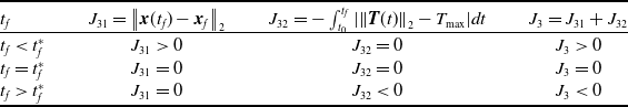
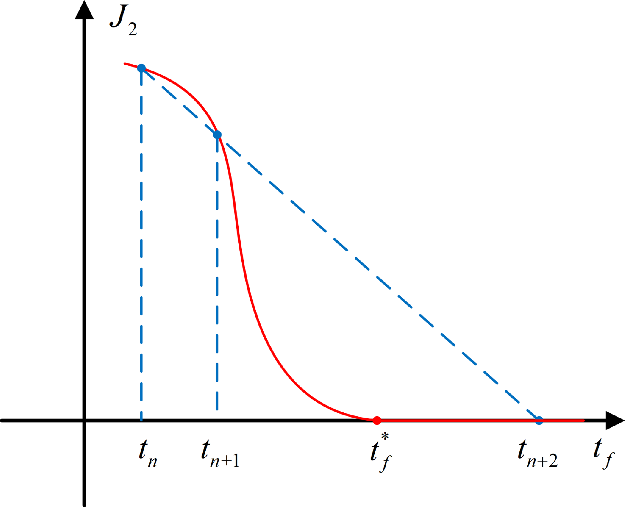
Figure 2. The iterative process of Newton’s method.
As shown in Fig. 3, the initial time-optimal problem is transformed into a double-layer optimisation framework, the inner layer is a convex programming problem, namely the minimum-terminal-error problem at given flight time, and the optimisation results are used to construct performance metric for outer layer root-finding problem. Furthermore, it’s worth distinguishing that J 2 denotes the optimisation objective for convex programming, while J 3 is only a performance metric constructed based on thrust and terminal error to guide the search for MFT.
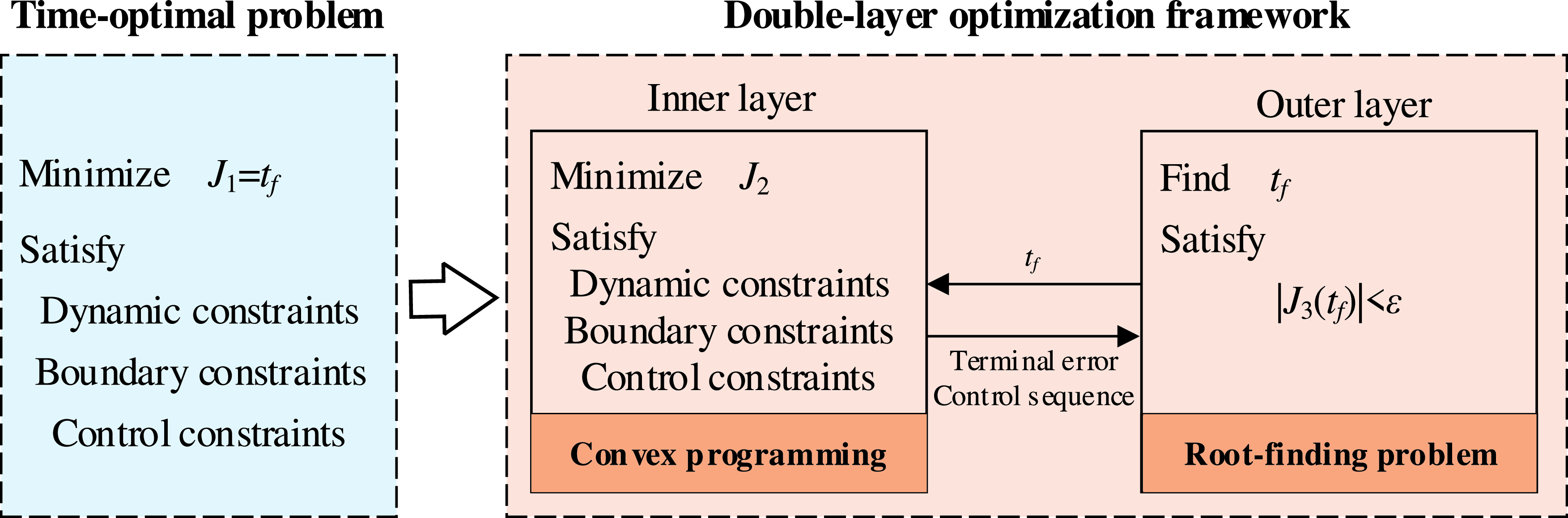
Figure 3. The double-layer optimisation framework.
4.0 The DNN-based rapid search method
In this section, the HSM combining bisection and Newton’s method is proposed to generate dataset for DNN training, and then a rapid search algorithm based on DNN is put forward to search for MFT.
4.1 Dataset generation and preprocessing
Based on Proposition 5, the time-optimal control problem has been transformed into a double-layer optimisation problem, where the outer layer can be solved by the iteration-based numerical method, such as the bisection method and Newton’s method. The bisection method repeatedly bisects the solution space and then selects subintervals in which the function changes signs until the convergence condition is satisfied. It’s robust and easy to implement, but computationally inefficient. On the contrary, the convergence of Newton’s method is quadratic, but it’s sensitive to initial points.
In view of this, we proposed the HSM that combines the advantage of both methods. The main idea is to reduce the solution space by the bisection method until the absolute function value of two boundary points is less than the preset value ${\bar J_3}$
and then the boundary points are used as starting points for Newton’s method. The bisection method provides a rough interval for Newton’s method to reduce iteration steps and thus improve robustness and calculation efficiency. The flowchart of HSM is concluded in Fig. 4.
${\bar J_3}$
and then the boundary points are used as starting points for Newton’s method. The bisection method provides a rough interval for Newton’s method to reduce iteration steps and thus improve robustness and calculation efficiency. The flowchart of HSM is concluded in Fig. 4.
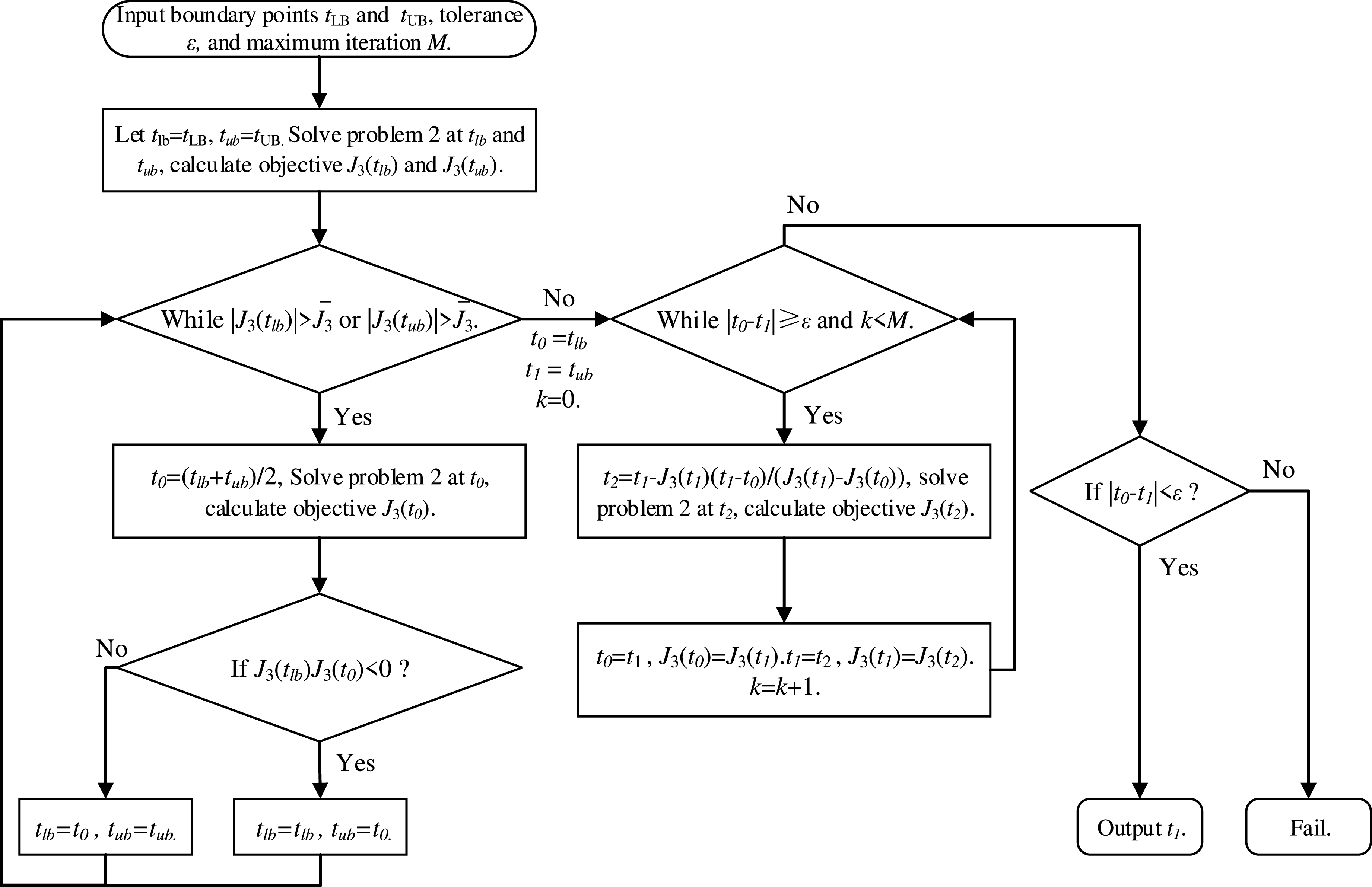
Figure 4. Flowchart of hybrid search method.
A dataset containing $5 \times {10^4}$
scenarios is randomly generated, and the MFT of each scenario is solved by the HSM. Assuming the chief spacecraft moves on 500km high circular orbit, the initial and final positions of deputy spacecraft are uniformly distributed within ±5km, and the initial and final velocities of deputy spacecraft are uniformly distributed within ±2m/s. Due to the large magnitude difference among the parameters, each parameter of the initial dataset is transformed into dimensionless values within
$5 \times {10^4}$
scenarios is randomly generated, and the MFT of each scenario is solved by the HSM. Assuming the chief spacecraft moves on 500km high circular orbit, the initial and final positions of deputy spacecraft are uniformly distributed within ±5km, and the initial and final velocities of deputy spacecraft are uniformly distributed within ±2m/s. Due to the large magnitude difference among the parameters, each parameter of the initial dataset is transformed into dimensionless values within $[0,1]$
by min-max normalisation.
$[0,1]$
by min-max normalisation.
 \begin{align}p' = \frac{{p - {p_{\min }}}}{{{p_{\max }} - {p_{\min }}}}\end{align}
where p is the initial parameter, ${p_{\min }}$
and
${p_{\min }}$
and ${p_{\max }}$
are the minimum and maximum values of each parameter,
${p_{\max }}$
are the minimum and maximum values of each parameter, $p'$
denotes the normalised parameter. The normalised dataset is divided into training datasets, validation datasets and test datasets in a ratio of 8:1:1. The three datasets are used to train the network, prevent overfitting and evaluate network performance, respectively.
$p'$
denotes the normalised parameter. The normalised dataset is divided into training datasets, validation datasets and test datasets in a ratio of 8:1:1. The three datasets are used to train the network, prevent overfitting and evaluate network performance, respectively.
4.2 Neural network design and training
The DNN consists of an input layer, an output layer and multiple hidden layers, each hidden layer contains multiple neurons. The dimensions of input and output layers are consistent with input and output data. In this paper, the sequence $[{x_0},{y_0},{z_0},{{\dot{\boldsymbol{x}}}_0},{{\dot{\boldsymbol{y}}}_0},{{\dot{\boldsymbol{z}}}_0},{x_f},{y_f},{z_f},{{\dot{\boldsymbol{x}}}_f},{{\dot{\boldsymbol{y}}}_f},{{\dot{\boldsymbol{z}}}_f}]$
consisting of the initial and final relative states is selected as the input of DNN and the MFT
$[{x_0},{y_0},{z_0},{{\dot{\boldsymbol{x}}}_0},{{\dot{\boldsymbol{y}}}_0},{{\dot{\boldsymbol{z}}}_0},{x_f},{y_f},{z_f},{{\dot{\boldsymbol{x}}}_f},{{\dot{\boldsymbol{y}}}_f},{{\dot{\boldsymbol{z}}}_f}]$
consisting of the initial and final relative states is selected as the input of DNN and the MFT $t_f^*$
as the output, the structure of DNN is shown in Fig. 5.
$t_f^*$
as the output, the structure of DNN is shown in Fig. 5.
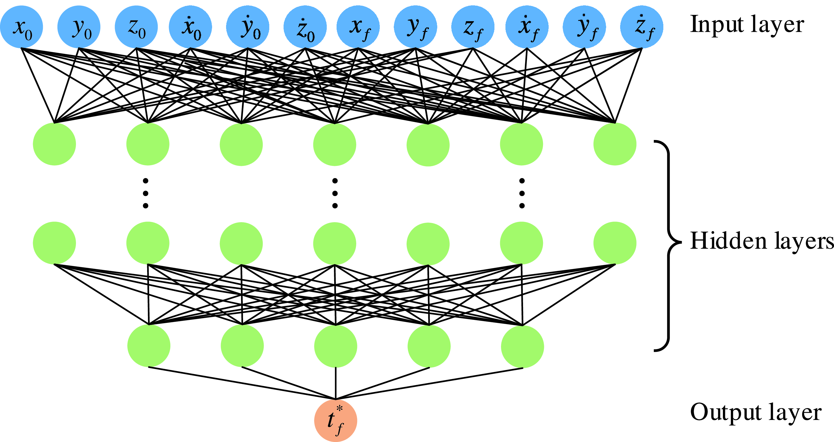
Figure 5. The structure of DNN.
The optimisation objective of neural network is the mean square error (MSE) between the training sample and the predicted value,
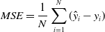 \begin{align}MSE = \frac{1}{N}\sum\limits_{i = 1}^N {({{\hat y}_i} - {y_i})} \end{align}
where N is the size of train dataset, ${y_i}$
and
${y_i}$
and ${\hat y_i}$
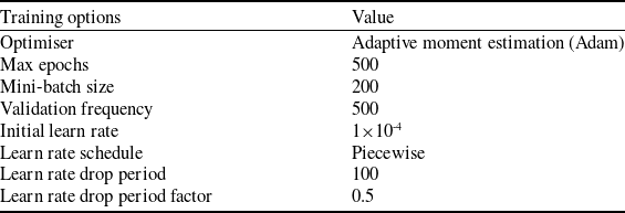
respectively represents real value and predicted value of DNN. The DNN training is based on deep learning toolbox built in MATLAB, the related training options are listed in Table 2.
${\hat y_i}$
respectively represents real value and predicted value of DNN. The DNN training is based on deep learning toolbox built in MATLAB, the related training options are listed in Table 2.
Table 2. The training options for DNN
The training process of four DNNs with different size is shown in Fig. 6, where the mark Net 7×50 indicates the number of hidden layers and neurons in hidden layer are 7 and 50. As shown in Fig. 6, the mean square error decreases rapidly with the increase of training steps, and finally fluctuates at the order of 10-4. In addition, the convergence speeds of Net 7×200 and Net 7×150 with larger network size are faster than that of Net 7×50 and Net 7×100.
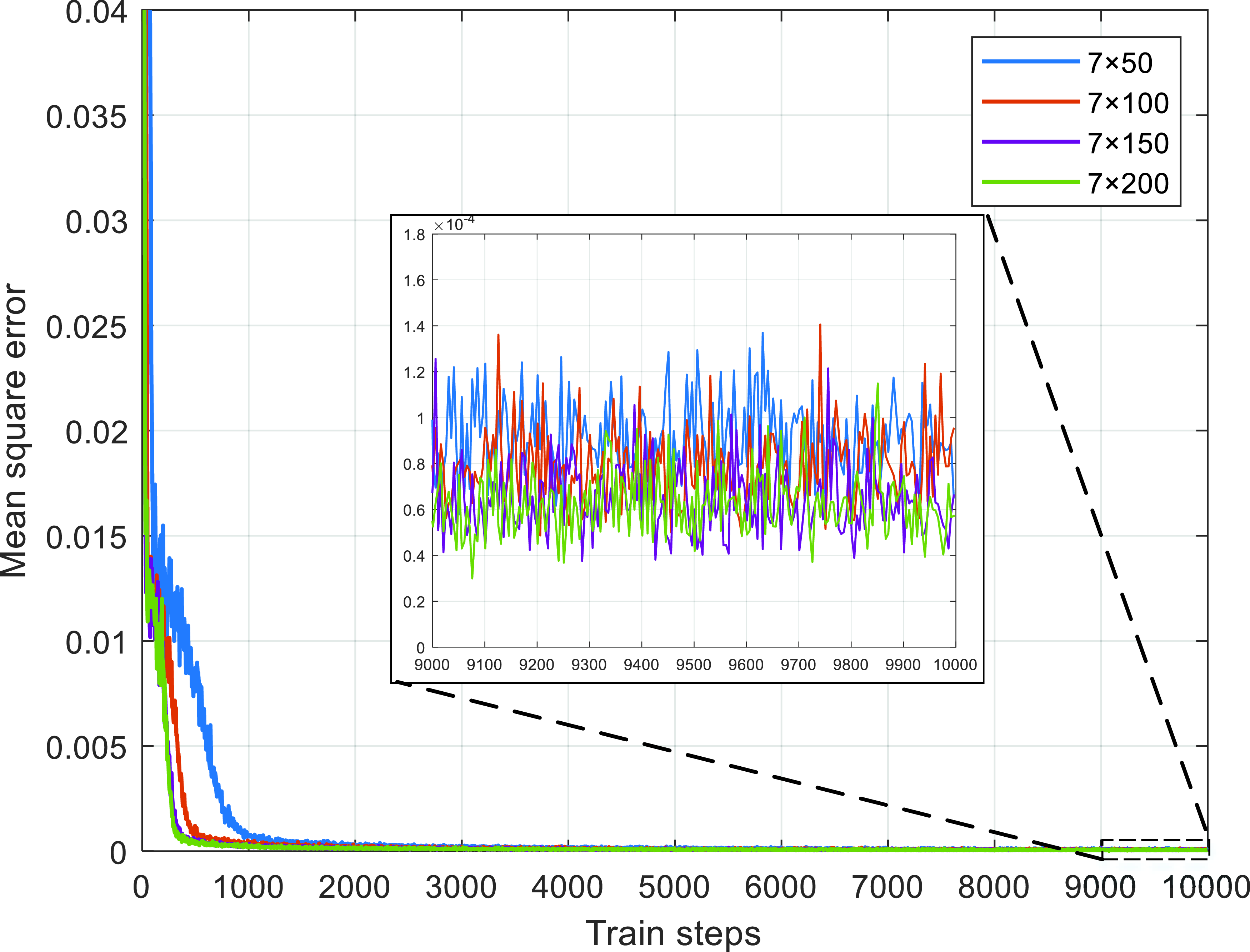
Figure 6. The training process of DNNs.
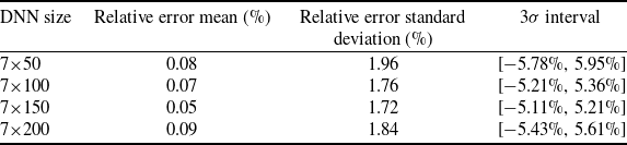
The performance of DNNs in test dataset is listed in Table 3. The relative error between real and predicted MFT follows the Gaussian distribution, and the mean of the relative error is approximately zero. With the increase of neurons, the standard deviation of relative error first decreases and then increases. The Net 7×150 performs well in both mean and standard deviation, and was selected to predicted MFT in the subsequent simulations. The 3σ interval of Net 7×150 is [-5.11%, 5.21%], namely the probability of relative error within this range is 99.73%.
Table 3. The relative error distribution of different DNNs
The performance of Net 7×150 in test dataset are shown in Fig. 7. It can be seen from Fig. 7(a) that the absolute error of predicted MFT obeys Gaussian distribution, most of the predicted errors are within 20s. As shown in Fig. 7(b), the predicted MFT (y axis) can fit real MFT (x axis) well, where the blue point and red line represent predicted MFT and reference line (y=x) respectively. Generating dataset and training DNNs took about 15 hours and 1 hour in a computer with Intel i7 processor and 16GB random access memory. Notably, the process of generating dataset and training the network can be implemented offline, and MFT will be predicted using trained DNN parameters online.
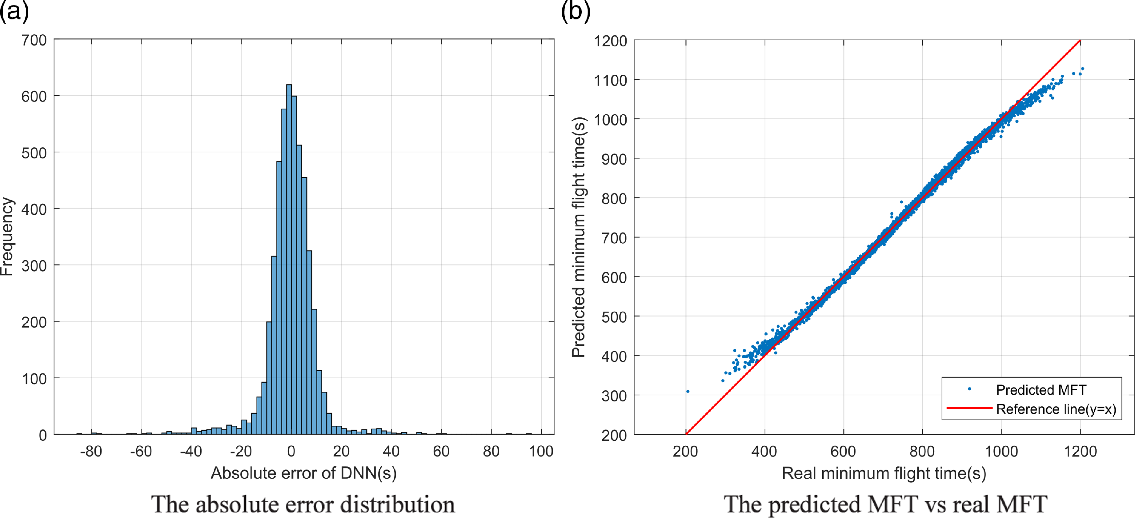
Figure 7. The performance of Net 7×150.
4.3 DNN-based rapid search method
The Newton’s method is sensitive to the initial point, high-quality initial points can ensure quadratic convergence, while poor initial points may lead to failure to converge. The proposed HSM takes the iterative result of the bisection method as the initial point of Newton’s method, which is robust but time-consuming.
Section 4.2 shows that the trained DNN can directly output the high-precision predicted value of MFT according to the initial and terminal boundary conditions. Although the predicted MFT cannot be directly applied to space tasks with high reliability requirements due to unavoidable errors, it can be taken as the initial points of Newton’s method, thus eliminating the binary inefficient search process and guaranteeing quadratic convergence of Newton’s method. The proposed DNN-RPM is robust and efficient, the diagram of HSM and DNN-RPM is shown in Fig. 8.
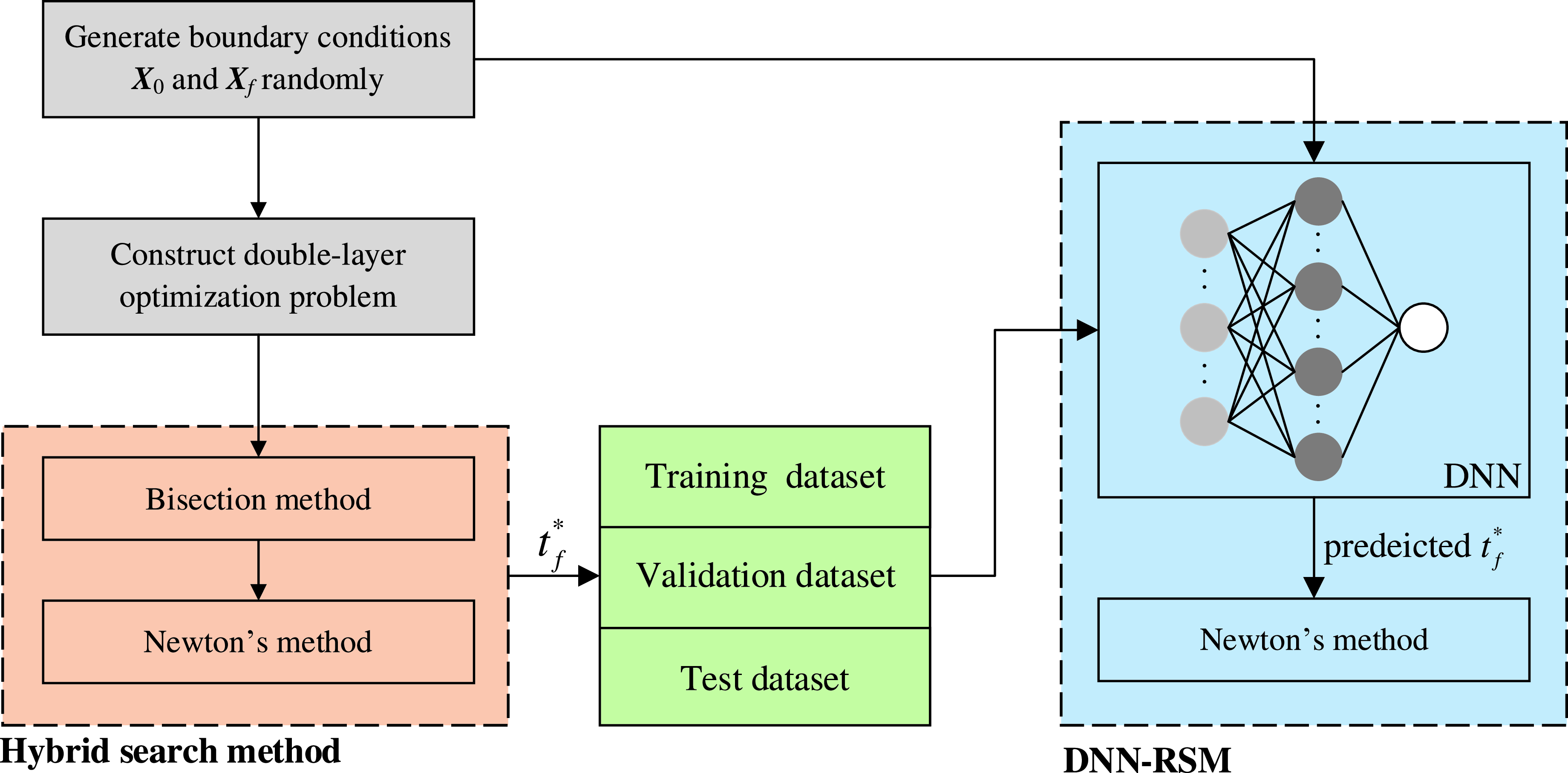
Figure 8. The diagram of HSM and DNN-RPM.
5.0 Numerical simulations
In this section, the HSM and DNN-RPM are firstly applied to generate time-optimal manoeuvering trajectory for single spacecraft, and the relevant properties of the time-optimal problem proved above are validated by simulation results. And then, the time-optimal NMC orbit injection problem is solved to validate the performance of proposed methods. Finally, three DNN-based strategies corresponding to different reliability are proposed to solve the minimum reconfiguration time of swarm.
Assuming that the chief spacecraft is in a 500km high near-circular orbit, the initial mass of each satellite in the swarm is 1,000kg. The maximum thrust and I
sp of the engine are 50N and 200s, respectively. The simulation process is discretised into 100 steps. Additionally, the tolerance and max iteration for HSM are 10−3 and 50, the preset ${\bar J_3} = 50$
, the lower and upper boundary of flight time are 100 and 3,000s. The CVX software is utilised to solve convex programming problem, where the SDPT3 is chosen as solvers, and other parameters remain the default setting. The numerical simulations are implemented on a computer with a 3.0GHz Intel Core i7 processor and 16GB random access memory.
${\bar J_3} = 50$
, the lower and upper boundary of flight time are 100 and 3,000s. The CVX software is utilised to solve convex programming problem, where the SDPT3 is chosen as solvers, and other parameters remain the default setting. The numerical simulations are implemented on a computer with a 3.0GHz Intel Core i7 processor and 16GB random access memory.
5.1 Time-optimal trajectory planning for spacecraft rendezvous
For time-optimal trajectory planning of single spacecraft, the initial and terminal relative states are set to X 0 =[103 m, 104 m, 0 m, 0 m/s, −2.21 m/s, 2.21 m/s]T, X f =[866.03 m, −103 m, 0 m, −0.55 m/s, −1.9 m/s, 0 m/s]T.
To begin with, the minimum terminal error problem (i.e., Problem 2) is solved with a given flight time, sampled every 10s between lower and upper boundary, and the performance index J 31, J 32 and J 3 are listed in Fig. 9. As defined in Section 3, the J 31 denotes the terminal error, J 32 is used to measure the difference between thrust curve and maximum thrust, and the J 3 is the sum of these two indexes. It can be seen from Fig. 9 that the optimal terminal error J 31 is larger than zero and decreases with time when t f <t f * , and it’s equal to zero when t f ≥t f * , which is consistent with Propositions 2 and 4. As proved in Proposition 3, the thrust magnitude remains T max when t f ≤t f * , and it’s less than T max when t f >t f * , the index J 32 is equal to zero in the first part but not in the second part. Therefore, the MFT for satellite manoeuvering is equal to the root of J 3.
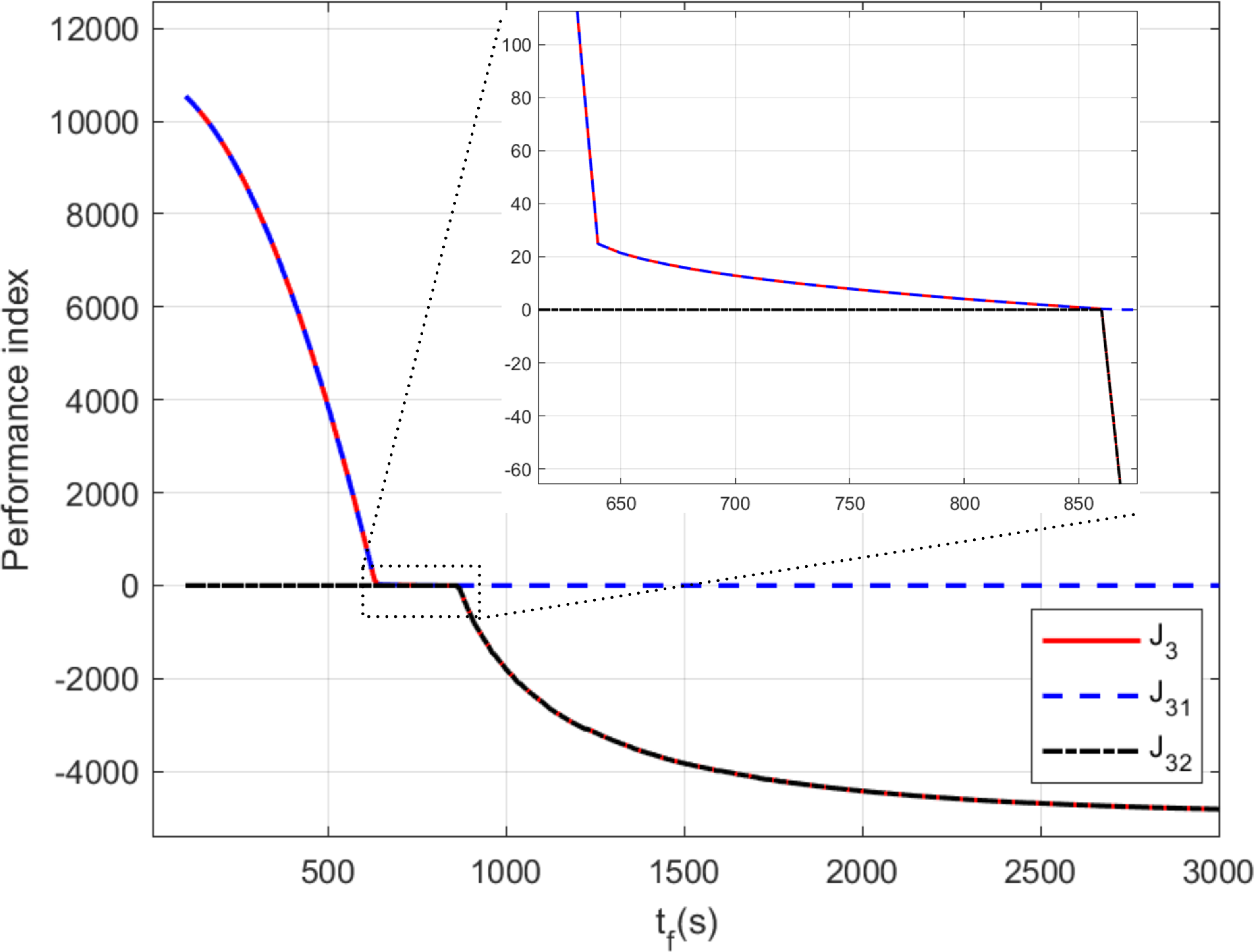
Figure 9. The performance index for different flight time.
And then, the time-optimal problem is solved with the proposed HSM and DNN-RPM, the relevant state and thrust curves are illustrated in Figs. 10–11. It can be seen from Fig. 10 that the proposed method can successfully generate transfer trajectory with the limitation of various constraints. As shown in Fig. 11, although the thrust components vary with time, the thrust magnitude remains at T max, which is consistent with Proposition 3.
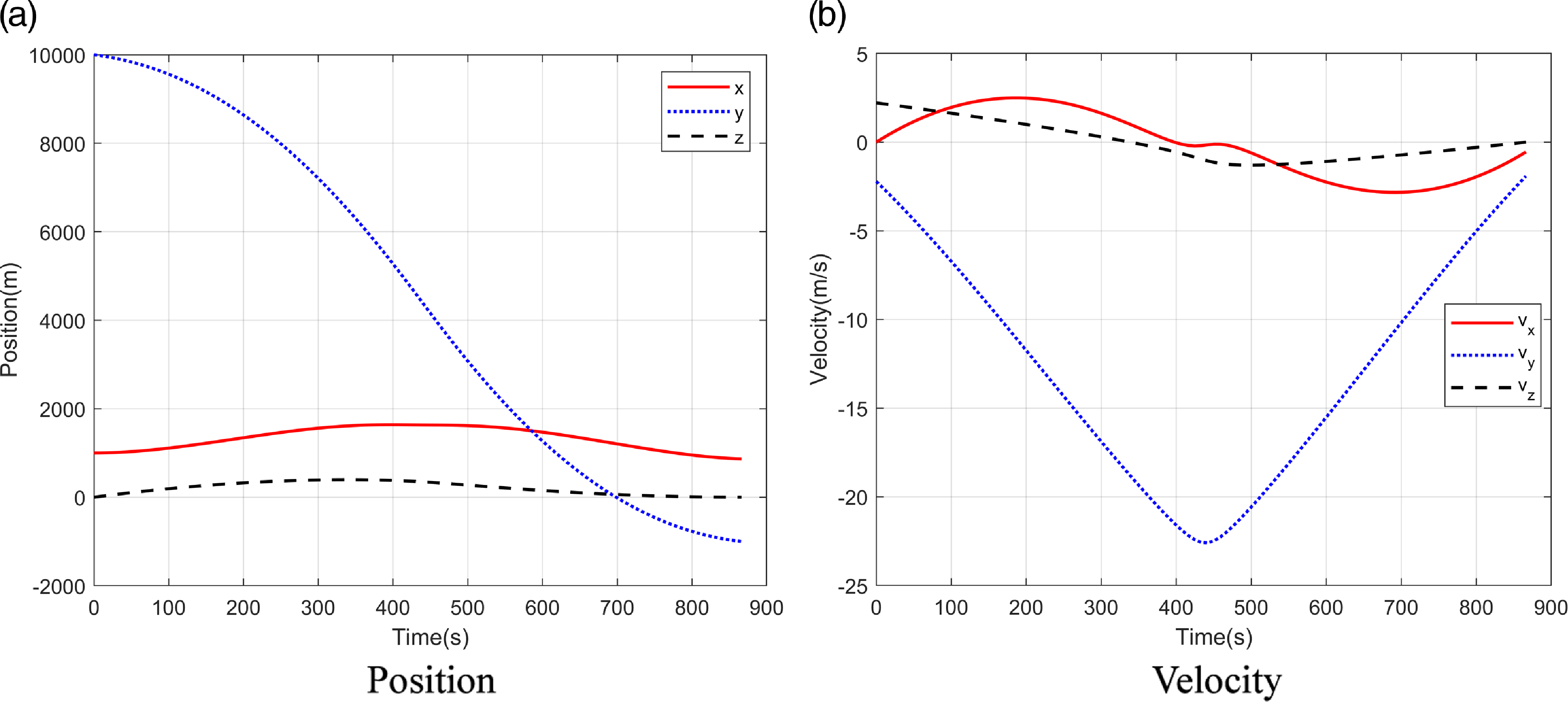
Figure 10. The time histories of state variables.
Furthermore, in order to evaluate the performance of the proposed methods, the time-optimal problem with the same configuration is also solved by the traditional bisection method, Newton’s method and sequential quadratic programming (SQP). The SQP method can be implemented by invoking the Fmincon function from Matlab optimisation toolbox directly, which is recognised as a powerful nonlinear programming solver. It’s worth noting that the first four methods solve the time-optimal problem based on convex programming, and the methods themselves are only used to search the MFT, while the SQP method optimises the control sequence and MFT simultaneously. Since the computational efficiency and convergence speed of SQP and traditional Newton’s method are greatly affected by initial value, these two methods are executed 50 times with random initial values. The performance comparison of different methods is listed in Table 4. Since the computing time of SQP is much larger than that of other methods, Fig. 12 only shows the computing time comparison of DNN-RPM, HSM, bisection method and Newton’s method.
Table 4. The performance metrics comparison
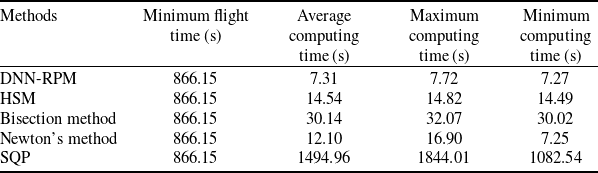
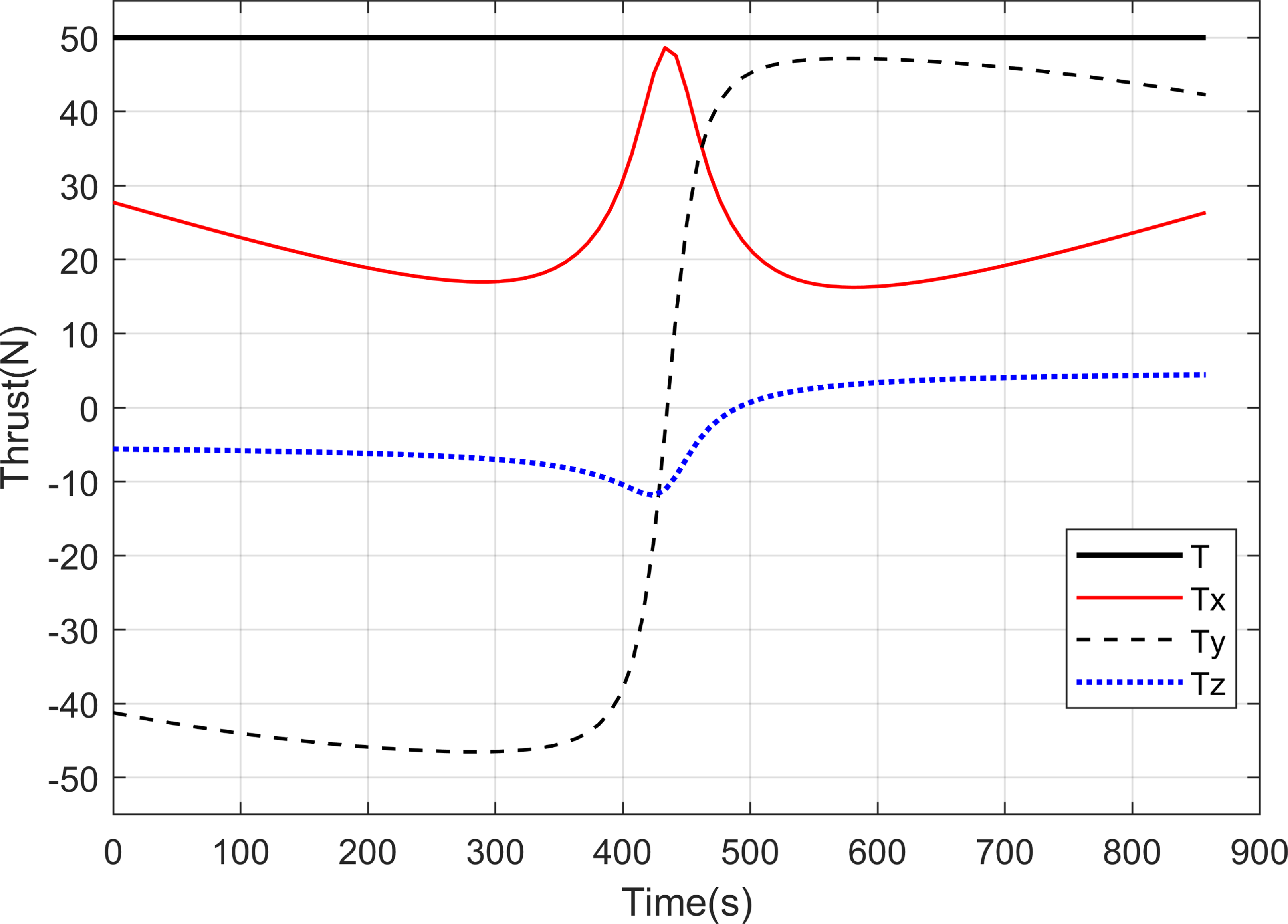
Figure 11. The time histories of thrust.
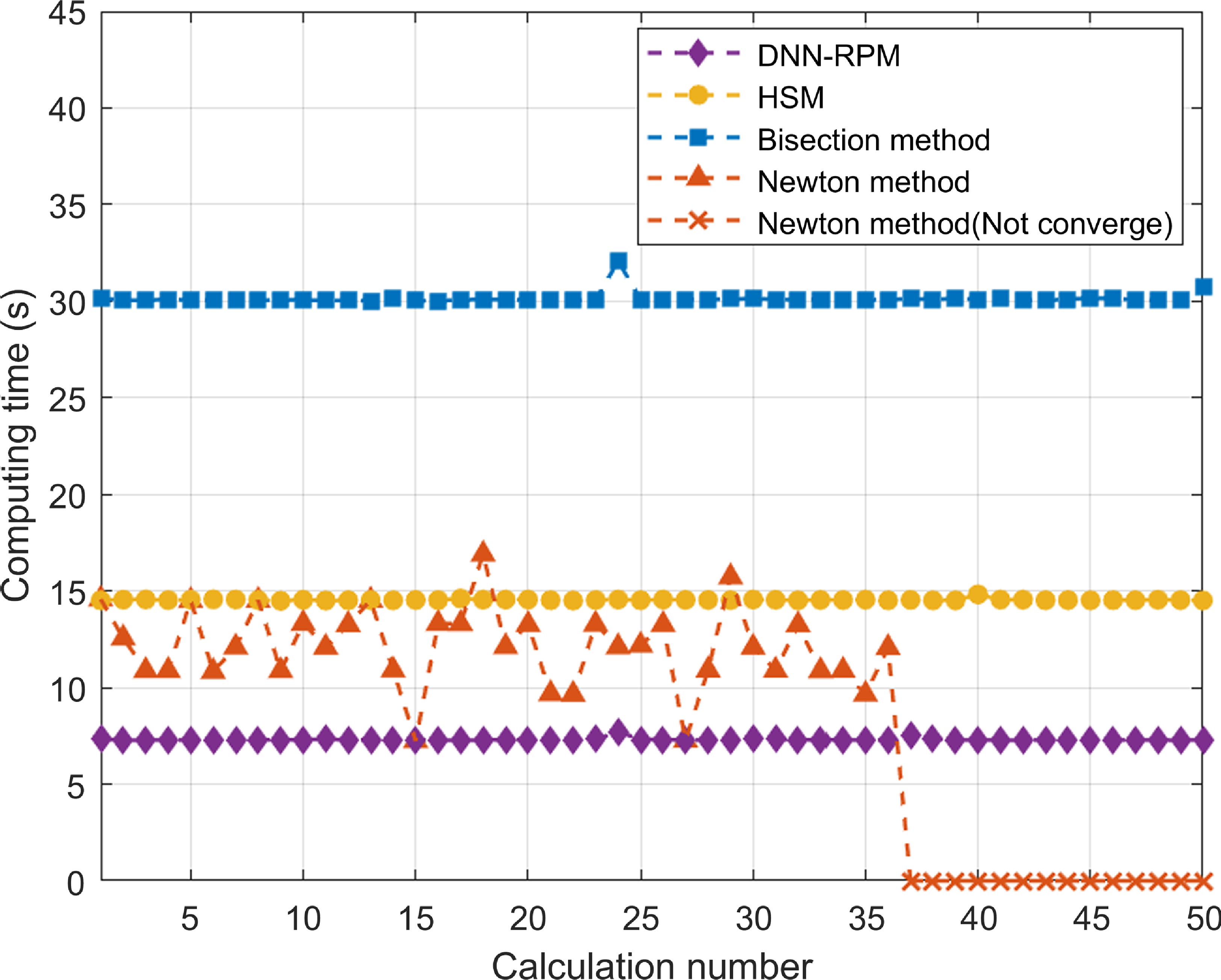
Figure 12. The computing time comparison.
It can be directly observed from Table 4 that the MFT obtained by the above five methods are almost the same. When it comes to the computation time criterion in Table 4, the first four methods take about two orders of magnitude less time than the SQP. Though the computation time could be affected by various factors like computer configuration and programme integration level, it shows the superiority of proposed double layer framework over nonlinear optimisation method in computational efficiency. The DNN-RPM takes 7.31s to calculate MFT, HSM takes about twice as long, and the bisection method takes about four times as long. As shown in Fig. 12 and Table 4, the traditional Newton’s method is slightly more computationally efficient than the HSM, but fails to converge in 14 out of 50 calculations. Therefore, the proposed DNN-RPM demonstrates its superiority in both computational efficiency and robustness.
5.2 Natural-motion circumnavigation injection
The NMC orbit, also known as passive relative orbit, is a kind of closed relative orbit where the deputy can fly around chief without extra fuel consumption [Reference Lu, Lewis, Adams, DeVore and Petersen28]. In order to form an NMC orbit, the secular term in y direction should be omitted,
 \begin{align}{\dot{\boldsymbol{y}}} = - 2nx\end{align}
The projection of the NMC orbit into x-y plane is a 2×1 ellipse, and the NMC orbit can be represented by a set of configuration parameters $[b,c,{y_c},\psi ,\phi ]$
. The conversion equation between relative states and NMC orbit configuration parameters is as follows,
$[b,c,{y_c},\psi ,\phi ]$
. The conversion equation between relative states and NMC orbit configuration parameters is as follows,
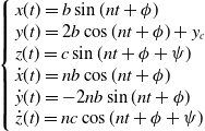 \begin{align}\left\{ \begin{array}{l}x(t) = b\sin (nt + \phi )\\y(t) = 2b\cos (nt + \phi ) + {y_c}\\z(t) = c\sin (nt + \phi + \psi )\\{\dot{x}(t)} = nb\cos (nt + \phi )\\{\dot{y}(t)} = - 2nb\sin (nt + \phi )\\{\dot{z}(t)} = nc\cos (nt + \phi + \psi )\end{array} \right.\end{align}
where b is the semi-minor axis of in-plane ellipse, y
c
is the displacement of in-plane ellipse centre in y-axis, c is the maximum displacement of NMC orbit in z-axis, $\phi $
and
$\phi $
and $\psi $
are phase angle of the in-plane and out-plane motion.
$\psi $
are phase angle of the in-plane and out-plane motion.
For the time-optimal NMC injection problem, the target is to find control vector
T
(t) and entering phase angle $\phi $
to minimise flight time and satisfy corresponding constraints. Compared with time-optimal trajectory planning for a single satellite, the NMC injection problem needs to optimise not only how to go (control vector), but also where to go (entering phase angle
$\phi $
to minimise flight time and satisfy corresponding constraints. Compared with time-optimal trajectory planning for a single satellite, the NMC injection problem needs to optimise not only how to go (control vector), but also where to go (entering phase angle $\phi $
), which greatly increases the difficulty of optimisation. In this case, the SQP algorithm is adopted to search entering phase angle
$\phi $
), which greatly increases the difficulty of optimisation. In this case, the SQP algorithm is adopted to search entering phase angle $\phi $
, the control vectors are generated by HSM and DNN-RPM, respectively.
$\phi $
, the control vectors are generated by HSM and DNN-RPM, respectively.
The NMC orbit configuration parameters are set to b=2,000m, c=2,000m, y
c=0m, $\psi = {\pi \mathord{\left/ {\vphantom {\pi 3}} \right.} 3}$
rad, the initial relative state of deputy satellite is
$\psi = {\pi \mathord{\left/ {\vphantom {\pi 3}} \right.} 3}$
rad, the initial relative state of deputy satellite is ${{X}_0} = {[5 \times {10^3}m,5 \times {10^3}m,\,5 \times {10^3}m,\,0{\textrm{ m/s}},\,0{\textrm{ m/s}},\,0{\textrm{ m/s}}]^T}$
. The simulation results are listed in Figs. 13–14 and Table 5.
${{X}_0} = {[5 \times {10^3}m,5 \times {10^3}m,\,5 \times {10^3}m,\,0{\textrm{ m/s}},\,0{\textrm{ m/s}},\,0{\textrm{ m/s}}]^T}$
. The simulation results are listed in Figs. 13–14 and Table 5.
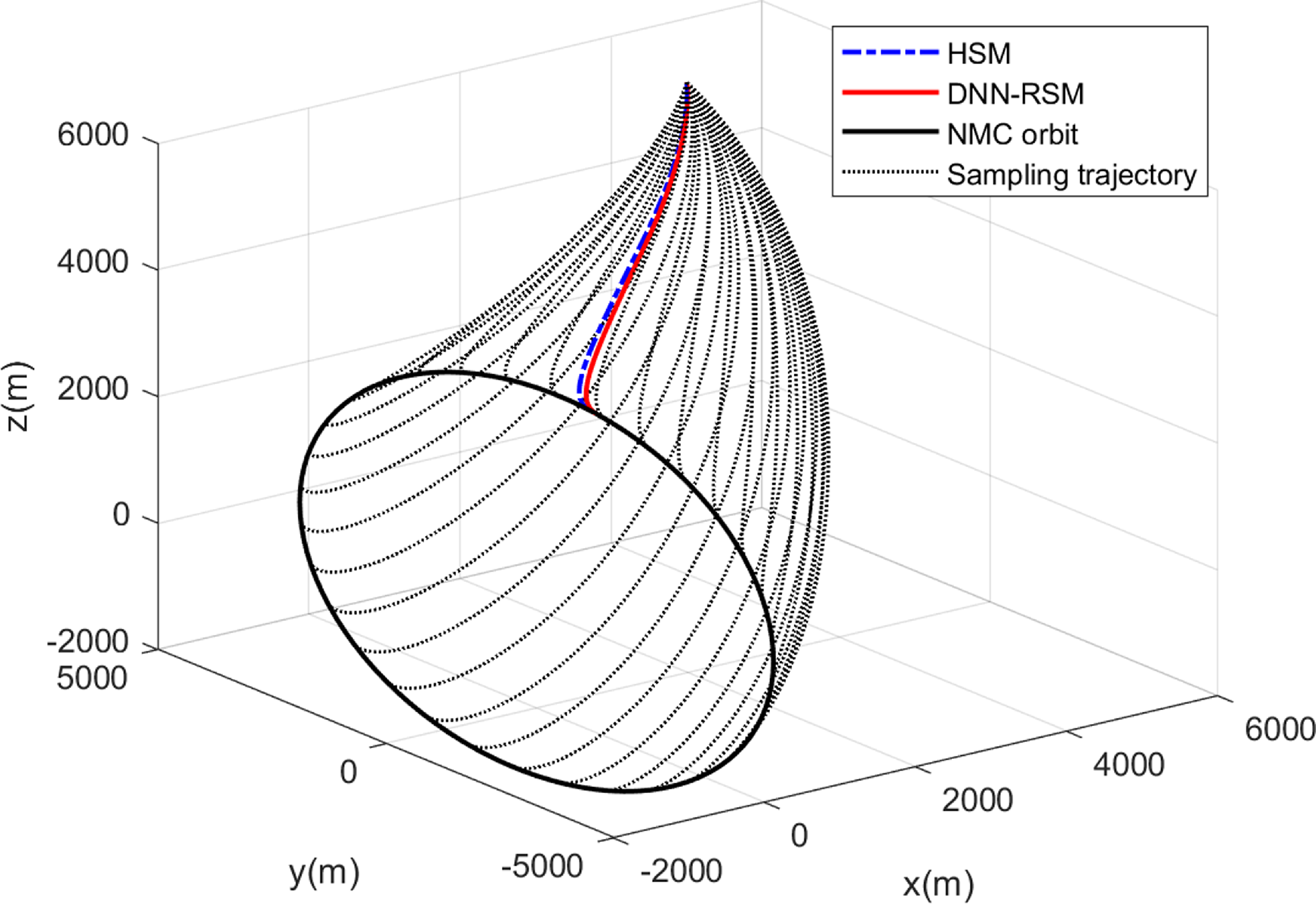
Figure 13. The manoeuvering trajectory of NMC injection.
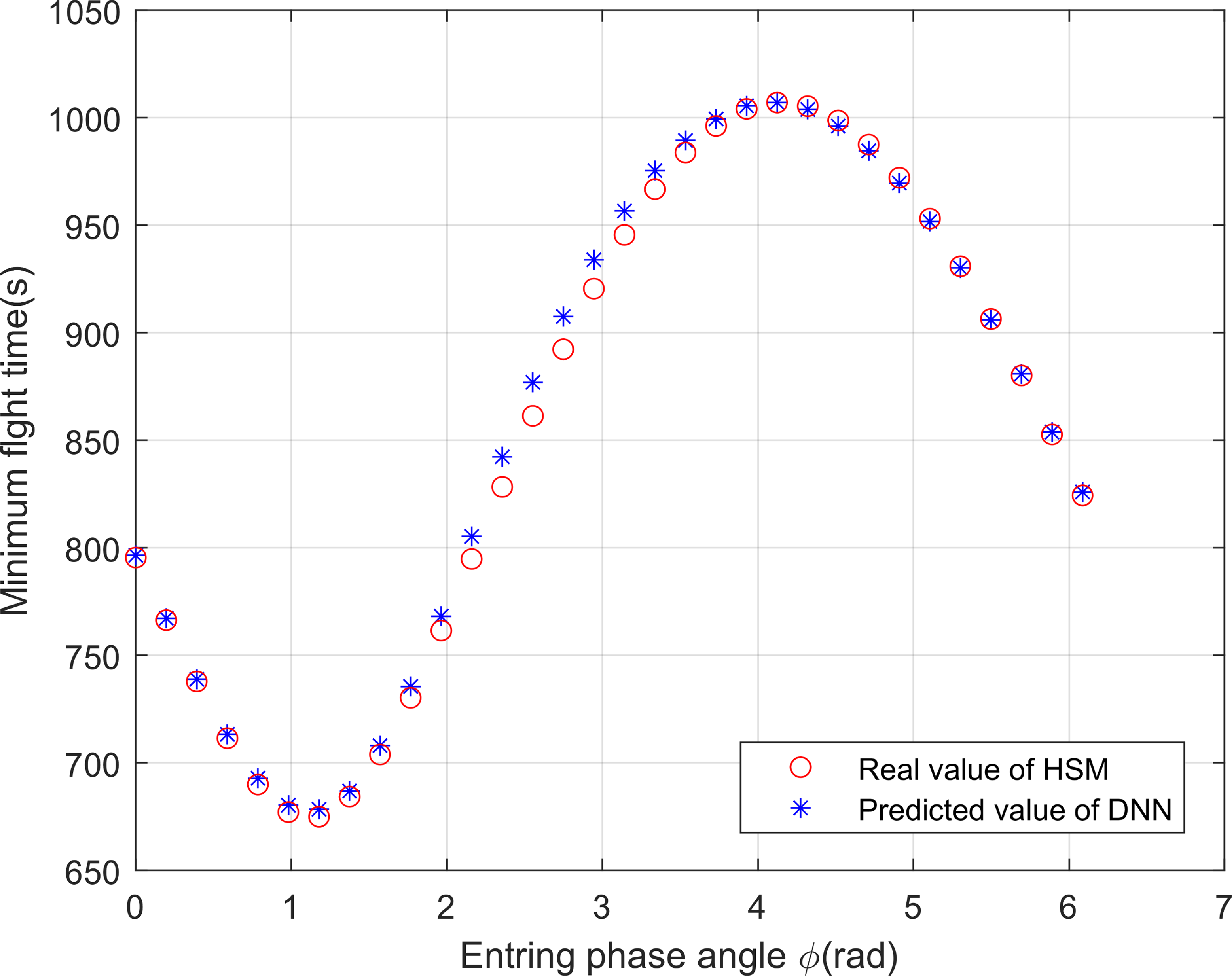
Figure 14. The minimum flight time generated by DNN and HSM.
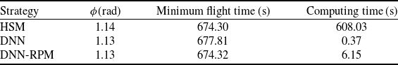
Table 5. The performance metrics of different strategies
As shown in Fig. 13, the red solid line and blue dotted line, respectively, represent the time-optimal injection trajectory generated by DNN-RPM and HSM, while the black line represents the NMC orbit. It can be directly observed that the time-optimal injection trajectories of DNN-RPM and HSM are close, which is consistent with the optimised entering phase angle in Table 5.
In addition, Fig. 13 shows the manoeuvering trajectories at 32 sampling points on the NMC orbit with black dot lines, and Fig. 14 demonstrates the MFTs predicted by DNN and calculated by HSM at each sampling point. The predicted MFTs at all sampling points are similar to the real MFTs, which again indicated the high prediction accuracy of DNN.
As shown in Table 5, the difference between the first strategy and the latter two lies in using the calculation result of HSM to guide SQP algorithm to search entering phase angle, rather than DNN’s predicted value. The entering phase angle calculated by HSM strategy and DNN strategy is very close, and the relative error is less than 1%. The DNN-RPM strategy takes the convergence entering phase angle of DNN strategy as the terminal state, and then calculates the MFT with DNN-RMS method. In other words, the flight time of 677.81 and 674.32s, respectively, represents the MFT predicted by DNN and calculated by DNN-RPM when entering phase angle $\phi $
=1.13rad. Additionally, the average computing time of HSM is 608.03 s, and that of DNN and DNN-RMS is 0.37 and 6.15s respectively. Due to the high computational efficiency of DNN, the computing time of DNN-RPM is about two orders of magnitude smaller than that of HSM.
$\phi $
=1.13rad. Additionally, the average computing time of HSM is 608.03 s, and that of DNN and DNN-RMS is 0.37 and 6.15s respectively. Due to the high computational efficiency of DNN, the computing time of DNN-RPM is about two orders of magnitude smaller than that of HSM.
5.3 The minimum reconfiguration time for swarm
Swarm reconfiguration is one of the enabling technologies for various space missions, which means that all spacecraft manoeuver from the initial states to the specified terminal states simultaneously. For a cluster containing Ns spacecraft, each spacecraft corresponds to an MFT, and the swarm reconfiguration time must be larger than $\max \{ MF{T_1},MF{T_2}, \cdots ,MF{T_{Ns}}\} $
to ensure that all spacecraft can generate feasible trajectories. Therefore,
$\max \{ MF{T_1},MF{T_2}, \cdots ,MF{T_{Ns}}\} $
to ensure that all spacecraft can generate feasible trajectories. Therefore, $\max \{ MF{T_1},MF{T_2}, \cdots ,MF{T_{Ns}}\} $
is regarded as the minimum reconfiguration time of spacecraft swarm in this section. To determine the minimum reconfiguration time, the simplest idea is to apply the above HSM or DNN-RPM to calculate the MFT of each spacecraft in turn, and take the maximum MFT as the minimum reconfiguration time of the whole swarm. However, this progress is time-consuming.
$\max \{ MF{T_1},MF{T_2}, \cdots ,MF{T_{Ns}}\} $
is regarded as the minimum reconfiguration time of spacecraft swarm in this section. To determine the minimum reconfiguration time, the simplest idea is to apply the above HSM or DNN-RPM to calculate the MFT of each spacecraft in turn, and take the maximum MFT as the minimum reconfiguration time of the whole swarm. However, this progress is time-consuming.
Three DNN-based strategies corresponding to different reliability are proposed, which are named high, medium and low reliability, respectively. The main difference among these three strategies is which spacecraft in the swarm should be chosen to calculate its real MFT. The high reliability strategy uses DNN-RPM to calculate the MFTs of all spacecraft in the swarm, and then takes the maximum MFT as the minimum reconfiguration time of the whole swarm. The low reliability strategy first predicts the MFTs of all spacecraft through DNN, and then calculates the real MFT of the slowest spacecraft by DNN-RPM as the minimum reconfiguration time.
For the medium reliability strategy, the MFTs of all spacecraft are firstly predicted by DNN, and then n-σ intervals of maximum MFT are taken as a filter, thus reducing call number of DNN-RPM. As shown in Fig. 15, the hexagons represent the predicted MFTs, and the I-boxes mean the responding n-σ intervals. Only one satellite’s n-σ interval intersects with that of the maximum predicted MFT in Fig. 15, so there is no need to calculate the real MFT of other satellites. According to the Gaussian distribution characteristics, when n is set to 1, 2 and 3, the reliability of this strategy is 68.27%, 95.45% and 99.73%. The difference among these three strategies is shown in Fig. 16.
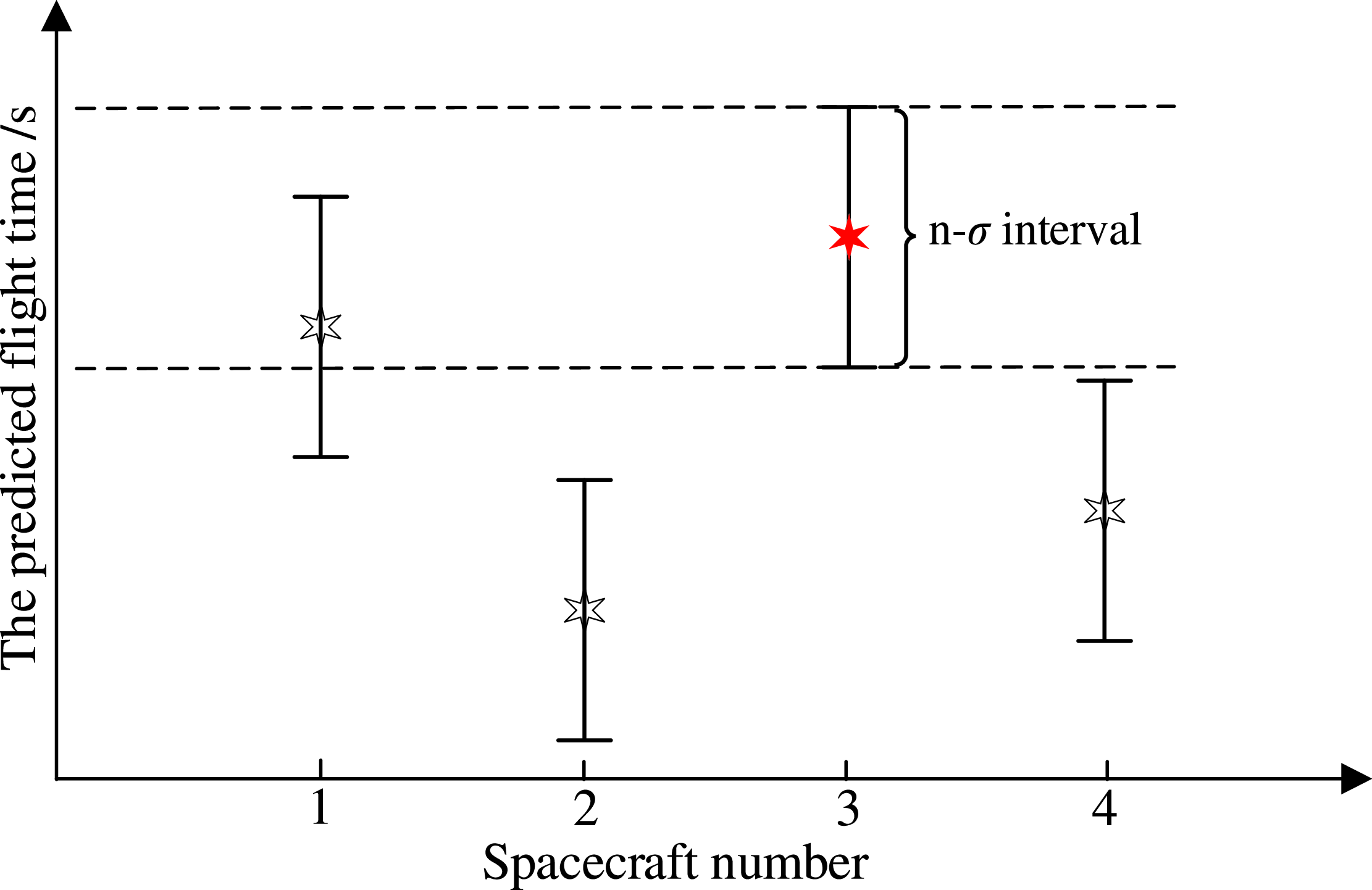
Figure 15. The n-σ intervals of predicted MFT.
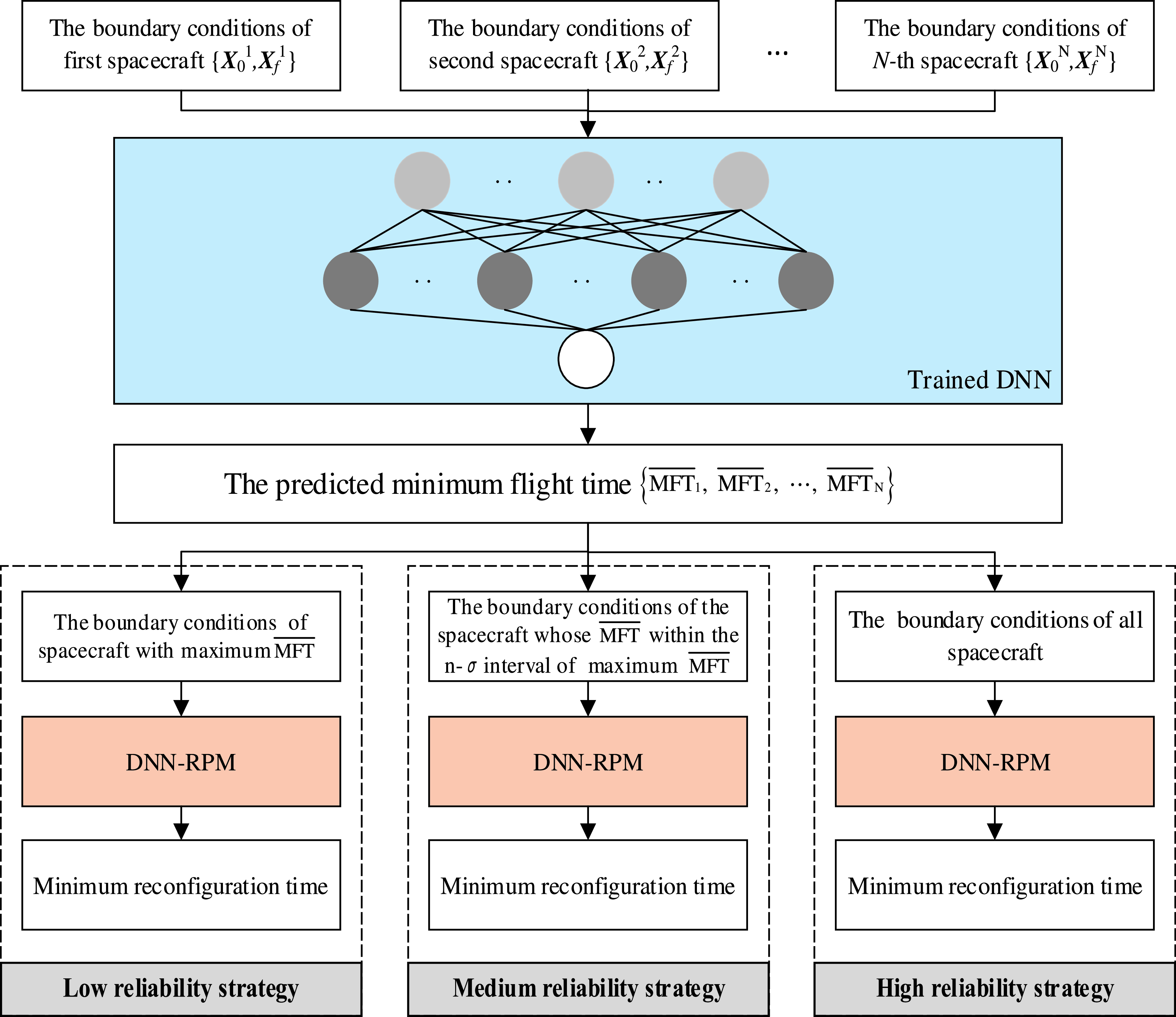
Figure 16. The diagram of low, medium and high reliability strategy.
The initial positions of swarm satellites are located on the eight corners of a 10km×10km× 10km cube centred at the chief in the LVLH frame, and the initial velocities are set to 0m/s. The terminal positions are uniformly distributed on an NMC orbit with b=2,000m, c=0m, y
c=0m, $\psi = \pi $
rad. The manoeuvering trajectories generated by DNN-RPM are presented in Fig. 17, and the computing time of four strategies are listed in Table 6.
$\psi = \pi $
rad. The manoeuvering trajectories generated by DNN-RPM are presented in Fig. 17, and the computing time of four strategies are listed in Table 6.
Table 6. The performance metrics of different strategies
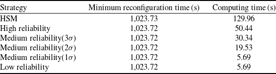
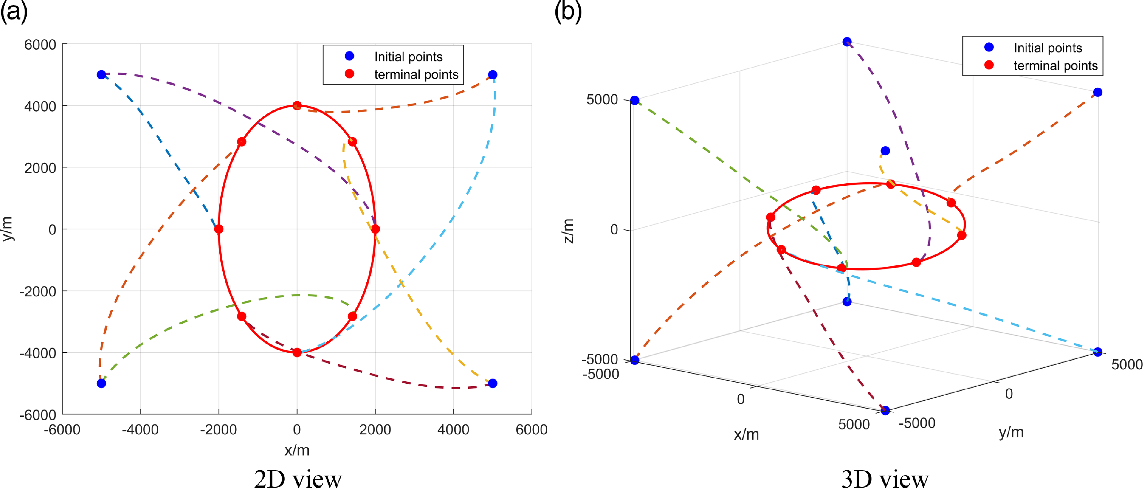
Figure 17. The manoeuvering trajectories of swarm reconfiguration.
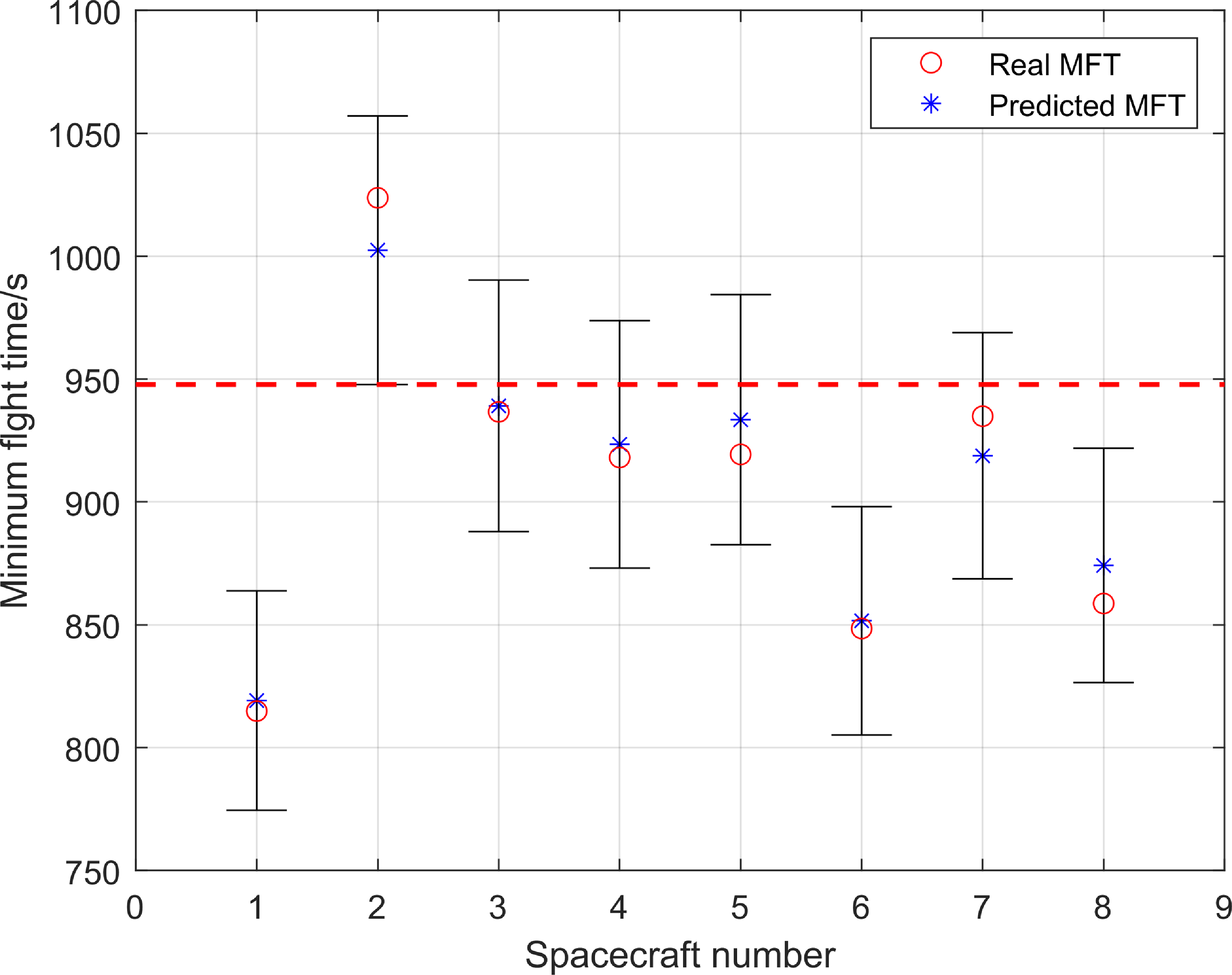
Figure 18. The predicted and real MFT of each spacecraft.
As shown in Table 6, the minimum reconfiguration times calculated by HSM and three DNN based strategies are similar, while the computing times are quite different. The first two strategies are based on the traversal idea and require calling HSM and DNN-RPM eight times, respectively. The difference in computing time of these two strategies depends on the calculation efficiency of HSM and DNN-RPM.
The medium reliability strategy uses the n-σ interval as a filter, thereby reducing call numbers of the underlying MFT optimisation methods. Taking 3σ interval for example, as shown in Fig. 18, red and blue marks represent the real and predicted MFTs of each spacecraft, and the black intervals are the corresponding 3σ intervals. The lower boundary of the 3σ interval of satellite 2 is larger than the upper boundary of spacecraft 1, 6 and 8. That is to say, the probability that the MFT of satellite 2 is larger than these spacecraft is 99.7%. Therefore, the process of calculating the accurate value of these spacecraft’s MFT can be omitted, and only need to call the DNN-RPM 5 times to calculate real MFTs of other spacecraft. Finally, the low reliability strategy only needs to call DNN-RMS once for calculating the MFT of the slowest spacecraft 2. When n is 1, 2 and 3, the number of calls of DNN-RPM is 1, 3 and 5, and the corresponding calculation time is 5.69, 19.53 and 30.34s.
In summary, the high reliability strategy can be used for tasks with high precision requirements, and the probability of obtaining optimal solution is 100%. The low reliability strategy is suitable for tasks with high timeliness requirements, so as to determine the minimum reconfiguration time as quickly as possible. As a compromise method, the medium reliability strategy can flexibly adjust the computing efficiency according to the reliability requirements.
It’s worth noting that the trajectories presented in Fig. 17 may not be the final feasible trajectories because the collision avoidance constraints are neglected during programming, but the minimum reconfiguration time obtained by those strategies is still reliable. Since the minimum reconfiguration time of is determined by the slowest satellite, the trajectory of the slowest satellite can be regarded as a reference trajectory, and then the collision avoidance constraints can be convexified and solved by sequential convex programming proposed in Ref. [Reference Morgan, Chung and Hadaegh8].
6.0 Conclusion
Concentrating on time-optimal trajectory planning for spacecraft rendezvous, this paper proposes a rapid trajectory planning method based on convex optimisation and deep neural network. The time-optimal control problem is transformed into convex form, and the thrust properties are analysed theoretically and validated numerically. The convexification technique can be extended to other time-optimal control problems. Compared with nonlinear optimisation method and traditional root-finding algorithm, the proposed DNN-RPM is capable of improving computational efficiency while ensuring algorithm robustness in generating time-optimal trajectory. For NMC orbit injection problem and swarm reconfiguration, the trained DNN can predict MFT with high precision, thus evidently reducing iteration steps and improving calculation efficiency. Future work will focus on improving the generalisation ability and prediction accuracy of DNN.
Competing interests
The author(s) declared no potential competing interests concerning the research, authorship and publication of this paper.


