


Nomenclature
- b
-
wing span; m
- c
-
wing chord, m
- ${\bar{\bar{c}}}$
-
mean aerodynamic chord, m
-
${C_D}$
-
drag coefficient
-
${C_L}$
-
lift coefficient
-
${C_l}$
-
rolling moment coefficient
-
$C'_{\!\!l}$
-
sectional lift coefficient
-
${C_{l\gamma }},{C_{l\xi}}$
-
roll control power for morphing and baseline configurations
- e
-
error
- h
-
height from ground to top of vertical tail in a stationary position, m
- K P, K I, K D
-
proportional, integral and derivative constants
- l
-
model length, m
- L e
-
length along wing span from tip, m
- m
-
model mass, kg
- p
-
roll rate, deg/s
- p’
-
non-dimensional roll rate
- P
-
pressure, Pa
- Ren
-
Reynolds number
- S
-
wing area, m
- t
-
time, s
- T
-
temperature, °C
- V
-
velocity, m/s
- y
-
distance along wing span from centreline, m


Greek symbols
- α
-
angle-of-attack, deg
- Δ
-
change or difference from mean unless otherwise indicated
- ξ
-
aileron deflection, deg
- γ
-
wing section twist, deg
- η
-
elevator deflection, deg
- ρ
-
density, kg/m3
- ζ
-
rudder deflection, deg
- ∑
-
sum
Subscripts
- i
-
i th chordwise wing location
- n
-
n th spanwise wing location
- m
-
manoeuvre
- max
-
maximum
- stall
-
stall conditions
- TRIM
-
aircraft trim condition
- RMS
-
root-mean square
- tip
-
wing tip location
- ∞
-
freestream conditions
1. Introduction
The increasing prevalence of Unmanned Aerial Vehicles (UAVs) into the defence and security sectors continues unabated. From the first platforms tasked solely with intelligence, surveillance and reconnaissance (ISR) [1]; to present day logistics support and offensive, weapon-capable variants [1]; to future sea and land-based vehicle concepts currently being developed [Reference Sepulveda and Smith2], UAVs are set to dominate forthcoming aerial doctrine. Of critical importance to their mission is the need for highly capable, efficient, and effective aerial systems that can travel further, persist longer, carry greater payload, and possess high manoeuvrability during execution of mission critical objectives. Civilian applications including law enforcement, search and rescue, agriculture and supply logistics are equally important. All these systems will be vital to preserving future defence, security and economic interests.
A ‘Morphing UAV’, or a UAV possessing the ability to seamlessly modify and adapt itself geometrically to changing conditions and requirements in flight, can offer several enhancements. Such platforms possess the ability to transform (in real-time) to an optimal configuration irrespective of flight condition leading to significantly improved vehicle performance and efficiency [Reference Pecora, Amoroso and Lecce3]. Unfortunately, within today’s modern flight environment, this capability remains technically challenging and still out of reach. This is borne about by a critical need for any prospective design to meet conflicting design requirements. Principally, it must be both structurally stiff (to resist loads) while also compliant (to allow change) [Reference Barbarino, Bilgen, Ajaj, Friswell and Inman4–Reference Weisshaar6]. Maintaining surface continuity before, during and after transition (to achieve best aerodynamic performance) further complicates this trade-off [Reference Barbarino, Bilgen, Ajaj, Friswell and Inman4, Reference Weisshaar6, Reference Reich and Sanders7].
If such challenges can be overcome however, the capability to morph promises a step change in aerial capability. Previous conceptual, laboratory and wind tunnel work on various fixed and rotary wing platforms, as well as limited full-scale flight testing, have established improvements in vehicle performance, efficiency, manoeuvrability [Reference Pecora, Amoroso and Lecce3–Reference Abdulrahim, Garcia, Ivey and Lind9], structural weight savings [Reference Pecora, Amoroso and Lecce3, Reference Miller5, Reference Sanders, Eastep and Forster8, Reference Pendleton, Bessette, Field, Miller and Griffin10], improved stability and gust load alleviation characteristics [Reference Barbarino, Bilgen, Ajaj, Friswell and Inman4, Reference Miller5], reduced manoeuvre loads [Reference Pecora, Amoroso and Lecce3, Reference Miller5, Reference Pendleton, Bessette, Field, Miller and Griffin10], better aeroelasticity capabilities [Reference Pecora, Amoroso and Lecce3] as well as enhanced redundancy via distributed actuation [Reference Pecora, Amoroso and Lecce3–Reference Weisshaar6]. Practicality remains the primary issue [Reference Barbarino, Bilgen, Ajaj, Friswell and Inman4, Reference Sanders, Eastep and Forster8].
One of the most effectual morphing ideas is ‘wing-warping’, or the ability to actively change the spanwise wing twist distribution (hereafter also referred to as Active Twist Control or ATC). The Wright flyer [Reference Culick11] demonstrated this most notably, but the advent of discrete control surfaces (or DCS - i.e. ailerons, elevators and rudder) soon superseded this technology as faster, more capable aircraft requiring stronger and stiffer structures were developed [Reference Vasista, Tong and Wong12]. DCS use is now almost universal. Despite their popularity however, DCS remain a sub-optimal solution. Deflection in flight often promotes premature flow separation (at the hinge line through strong adverse pressure gradient development) reducing overall effectiveness and efficiency [Reference Barbarino, Bilgen, Ajaj, Friswell and Inman4, Reference Sanders, Eastep and Forster8, Reference Scherer13]. Significant complexity [Reference Vos, de Breuker, Barrett and Tiso14, Reference Amendola, Dimino, Magnifico and Pecora15], increased weight [Reference Pecora, Amoroso and Lecce3, Reference Miller5, Reference Pendleton, Bessette, Field, Miller and Griffin10, Reference Vos, de Breuker, Barrett and Tiso14, Reference Amendola, Dimino, Magnifico and Pecora15] and susceptibility to aeroelastic divergence are further deficiencies [Reference Pecora, Amoroso and Lecce3, Reference Miller5, Reference Voracek, Pendleton, Reichenbach, Griffin and Welch16].
Many of these problems are overcome with ATC. Moreover, while the effectiveness of ATC for attitude control is well-known, other equally transformative benefits are yet to be fully exploited. Among the most significant is the ability to tailor and optimise spanwise wing twist (and therefore the lift distribution) to meet differing flight conditions and mission requirements [Reference Pecora, Amoroso and Lecce3, Reference Abdulrahim, Garcia, Ivey and Lind9, Reference Pendleton, Bessette, Field, Miller and Griffin10, Reference Phillips, Fugal and Spall17]. Current fixed-wing aircraft possess only a limited ability to achieve such capabilities, with an overall design typically neither optimal nor ideal, but based on a set of concessions within broader operational needs [Reference Barbarino, Bilgen, Ajaj, Friswell and Inman4, Reference Stanewsky18, Reference Moorhouse, Sanders, Spakovsky and Butt19]. Given any increase in lift-to-drag ratio represents commensurate increases in range and endurance [Reference Phillips20], saves otherwise used fuel, ultimately reducing operational costs, maximising this capability could represent a potentially disruptive advance in achievable aerial effectiveness. This paper will assess this capability using an ATC technology applied to a small-scale UAV platform within a wind tunnel environment. The initial design rational, development and integration are all considered, with performance and control benefits against an unmodified baseline, quantified and evaluated.
2. The active twist control concept
The basic premise of the ATC concept used (Fig. 1) is to construct a portion of the wing using multiple, small thickness, rigid rib sections, positioned directly adjacent, that are free to rotate relative to one another. This relative movement facilitates the change in twist distribution over the combined assembly while maintaining a rigid and smooth surface. Internally, the structure also incorporates multiple span-wise rods (front and rear indicated) positioned around the periphery of each rib profile providing structural stiffness, rib alignment and edge surface continuity. In the initial embodiment from a previous preliminary investigation [Reference Kaygan and Gatto21] highlighted in Fig. 1, a servo-driven torque tube positioned at the quarter chord provided twist actuation. This tube was connected to a terminating wing-tip end section that transferred torque to all subsequent inboard elements. Overall, this initial work demonstrated suitability for purpose with application within a realistic flight environment also validated [22].

Figure 1. Details of the initial ATC concept developed including a close-up view (Detail A) of how the individual rib sections are assembled [Reference Kaygan and Gatto21].
3. Morphing UAV design, setup, and configuration
3.1. Baseline UAV platform
The UAV platform chosen as the baseline for this work was an Extreme Flight© Extra 300 EXP manufactured by Extreme Flight RC© [23] shown in Fig. 2. The model has a wingspan of 1320mm (52 inches), length of 1302mm, and a nominal flying mass, depending on setup, of between 1.7 and 1.8kg. The model is constructed from interlocking laser cut balsawood and plywood, carbon longerons, fibreglass and a carbon U-channel landing gear. It is classified as an ‘aerobatic’ model aircraft with a wide range of capabilities up to and including aggressive flight manoeuvring. The ailerons extend up to 90% of the semi-span ( $\thickapprox$
47% max chord ratio) with full span elevators (
$\thickapprox$
47% max chord ratio) with full span elevators ( $\thickapprox$
41% max chord ratio) and rudder (
$\thickapprox$
41% max chord ratio) and rudder ( $\thickapprox$
41% max chord ratio); both the latter incorporating an unshielded horn balance. Primary propulsion is provided by a 14x7 Xor© propellerFootnote
1
and Xpwr© T3910 motorFootnote
2
combination connected to an Airboss© 80 Electronic Speed ControllerFootnote
3
(ESC) with an Overlander© 4S 2500-3300 mAh LiPo batteryFootnote
4
used for primary electromotive potential. Four Hitec HS-5087MH micro servosFootnote
5
provide elevator, aileron and rudder deflection for primary flight control with the model chosen primarily based upon; (1) adequate size requirements for wind tunnel testing; (2) relative ease of modification, and; (3) the ability for assessment over a wide range of flight manoeuvres. Table 1 provides a summary of baseline characteristics with further details available from [23]. This information, together with more detailed measurements, were used to construct a Computer Aided Design (CAD) model for subsequent use within the design process.
$\thickapprox$
41% max chord ratio); both the latter incorporating an unshielded horn balance. Primary propulsion is provided by a 14x7 Xor© propellerFootnote
1
and Xpwr© T3910 motorFootnote
2
combination connected to an Airboss© 80 Electronic Speed ControllerFootnote
3
(ESC) with an Overlander© 4S 2500-3300 mAh LiPo batteryFootnote
4
used for primary electromotive potential. Four Hitec HS-5087MH micro servosFootnote
5
provide elevator, aileron and rudder deflection for primary flight control with the model chosen primarily based upon; (1) adequate size requirements for wind tunnel testing; (2) relative ease of modification, and; (3) the ability for assessment over a wide range of flight manoeuvres. Table 1 provides a summary of baseline characteristics with further details available from [23]. This information, together with more detailed measurements, were used to construct a Computer Aided Design (CAD) model for subsequent use within the design process.

Figure 2. Baseline UAV platform chosen [23].
Table 1. List of UAV baseline dimensions and characteristics used for analysis

3.2. Morphing UAV prototype design
3.2.1. Computational setup, analysis and validation
The design of the morphing UAV involved adoption of several computational tools to predict probable aerodynamic and structural performance metrics. ANSYS Fluent© and Athena Vortex lattice [Reference Drela and Youngren24] were the two main aerodynamic tools used; the former primarily to calibrate, verify and validate the latter, with ANSYS© workbench used for estimating structural loads and deflection magnitudes. Several design iterations encompassing both steps were employed to achieve the final configuration presented.
The first step in the design process was to obtain basic aerodynamic characteristics of the baseline model using CFD. This analysis was conducted in ANSYS Fluent© and utilised a steady-state Reynolds-Averaged Navier-Stokes solution (RANS) incorporating the k-ε realisable closure model (with enhanced wall treatment) conducted at standard sea-level conditions (ρ = 1.225kg/m3, P ∞ = 101.325kPa, T ∞ = 15°C). The freestream velocity was set to V ∞ = 30m/s for all computations using a velocity inlet condition with a pressure outlet at flow exit also specified. A second-order upwind spatial discretisation scheme with SIMPLEC pressure-velocity coupling was also used.
A hybrid mesh encompassing both structured hexahedral and unstructured triangular elements was constructed; the former used primarily adjacent to model surfaces to adequately resolve the boundary layer (y+ $\thickapprox$
1), with the latter, to characterise the wider external flow field. The model was positioned centrally within a rectangular cuboid farfield geometry 7.5b wide, 7.5b high, and 15b long, with the model spinner located 3.75b downstream of the inlet. No attempt was made to model the propeller geometry resulting in relevant wake effects being excluded. All model surfaces were specified as no-slip, with farfield walls given zero shear to negate the need to resolve the boundary layer reducing the number of elements required. The final grid configuration used was selected after a grid refinement study where both half and double that of the final element density selected (
$\thickapprox$
1), with the latter, to characterise the wider external flow field. The model was positioned centrally within a rectangular cuboid farfield geometry 7.5b wide, 7.5b high, and 15b long, with the model spinner located 3.75b downstream of the inlet. No attempt was made to model the propeller geometry resulting in relevant wake effects being excluded. All model surfaces were specified as no-slip, with farfield walls given zero shear to negate the need to resolve the boundary layer reducing the number of elements required. The final grid configuration used was selected after a grid refinement study where both half and double that of the final element density selected ( $\thickapprox$
5 million) and farfield geometry size indicated both C
D and C
L variation of less than 1%; this typically occurring after less than 4,000 iterations. To assess change in angle-of-attack, the model was first rotated about its lateral axis before reconstructing the grid (freestream velocity being aligned to the farfield axial geometry). The angle-of-attack range considered extended from 0° ≤ α ≤ 20° (Δα = 4°) with Fig. 3 providing grid detail (y = 0 – Fig. 3(a)) as well as an example surface pressure coefficient distribution at α = 4° (Fig. 3(b)).
$\thickapprox$
5 million) and farfield geometry size indicated both C
D and C
L variation of less than 1%; this typically occurring after less than 4,000 iterations. To assess change in angle-of-attack, the model was first rotated about its lateral axis before reconstructing the grid (freestream velocity being aligned to the farfield axial geometry). The angle-of-attack range considered extended from 0° ≤ α ≤ 20° (Δα = 4°) with Fig. 3 providing grid detail (y = 0 – Fig. 3(a)) as well as an example surface pressure coefficient distribution at α = 4° (Fig. 3(b)).

Figure 3. Baseline CFD at α = 4°; (a) Indicative grid slice at y = 0; (b) Surface pressure distribution.
AVL [Reference Drela and Youngren24] was used hereafter as the main aerodynamic design tool. This vortex lattice code provides both flight performance and mechanics predictions modelling lifting surfaces via an array of distributed horseshoe vortices on appropriately segmented panels. Various metrics are available using this code, however, estimating C D requires a supplementary source for zero-lift drag coefficient (C Do) [Reference Drela and Youngren24, Reference Stanford, Abdulrahim, Lind and Ifju25]. This was supplied by the CFD discussed above. Each lifting surface was nominally segregated into 20 spanwise and 20 chordwise panels with a non-linear bias distribution towards external edges. Given AVL solution fidelity also tends to be more uncertain with fuselage inclusion [Reference Drela and Youngren24], this influence was omitted (all surfaces were modelled as continuous across the symmetry plane). The flowfield is quasi-steady with similar flight conditions to those used in the CFD adopted (0° ≤ α ≤ 16°, Δα = 4°). The final AVL model used is shown in Fig. 4. Subsequent comparisons between CFD and AVL analyses provided in Fig. 5 show generally good agreement up to α = 16°, with the latter over-predicting C L by a maximum of 9%, and underpredicting C D by 8%. This behaviour was somewhat expected given the limitations of AVL to adequately resolve flow separation [Reference Drela and Youngren24].

Figure 4. Layout of AVL model used.

Figure 5. Comparison between Fluent and AVL baseline models; (a) C D, (b) C L.
3.3. Spanwise influence of morphing wing twist
To determine overall morphing configuration layout and dimensions along with baseline performance for comparisons, both morphing and baseline AVL models were developed; the former using an imposed linear wing twist spanwise distribution similar to [Reference Pecora, Amoroso and Lecce3], and the latter, embedded Ailerons, for roll control. For the former, Fig. 6 along with Table 2 quantifies the influence of wing segment length (L
e – see Fig. 6(b)) against calculated non-dimensional roll rate (ṕ = pb/(2V)) with a maximum γ = 16° deflection at the wing tip (aircraft trimmed about all 6 degrees of freedom). A design point of ṕ = 0.07 ( $\thickapprox$
180 deg/s) was chosen as a roll performance metric for both as this was expected to adequately demonstrate expected ATC capabilities as well as being approximately aligned with other typical aircraft configurations requiring aggressive manoeuvrability [Reference Miller5, Reference Chen, Sarhaddi, Jha, Liu, Griffin and Yurkovich26]. Figure 6 indicates L
e = 176mm achieves this level with the corresponding sectional lift coefficient distribution (αTRIM
$\thickapprox$
180 deg/s) was chosen as a roll performance metric for both as this was expected to adequately demonstrate expected ATC capabilities as well as being approximately aligned with other typical aircraft configurations requiring aggressive manoeuvrability [Reference Miller5, Reference Chen, Sarhaddi, Jha, Liu, Griffin and Yurkovich26]. Figure 6 indicates L
e = 176mm achieves this level with the corresponding sectional lift coefficient distribution (αTRIM $\thickapprox$
1.13°) provided by AVL for both configurations highlighted in Figs. 7 and 8. These results show the clear differences in how differential lift production via the dissimilar sectional lift topologies generate rolling moment; morphing twist being concentrated at the wing tips, and ailerons of the baseline having a much more distributed impact. This comparison also allows a correlation between the two, providing an equivalent aileron deflection for comparable wing twist performance. These results are presented in Table 2 and show under these conditions that for L
e = 176mm with γtip = 16° is equivalent to ξ = 3.52°. Along with this comparison, additional spanwise locations were also calculated (L
e2 = 267mm, L
e3 = 367mm) and are also included in Table 2 and Fig. 6 to allow the ability for further enhanced roll control as well as localised spanwise adjustment and control of the lift distribution [Reference Phillips, Fugal and Spall17, Reference Stanford, Abdulrahim, Lind and Ifju25]. These additional segment lengths were selected based on an iterative design loop tasked with minimising the number of spanwise actuation stations (to minimise weight and complexity) whilst maximising structural rigidity under aerodynamic loading. With all these three stations acting in unison with γtip = 16°, predicted roll performance significantly improves to |ṕ| = 0.163, equivalent to a baseline aileron deflection of ξ = 8.21°. A similar trend has been observed previously [Reference Abdulrahim, Garcia, Ivey and Lind9].
$\thickapprox$
1.13°) provided by AVL for both configurations highlighted in Figs. 7 and 8. These results show the clear differences in how differential lift production via the dissimilar sectional lift topologies generate rolling moment; morphing twist being concentrated at the wing tips, and ailerons of the baseline having a much more distributed impact. This comparison also allows a correlation between the two, providing an equivalent aileron deflection for comparable wing twist performance. These results are presented in Table 2 and show under these conditions that for L
e = 176mm with γtip = 16° is equivalent to ξ = 3.52°. Along with this comparison, additional spanwise locations were also calculated (L
e2 = 267mm, L
e3 = 367mm) and are also included in Table 2 and Fig. 6 to allow the ability for further enhanced roll control as well as localised spanwise adjustment and control of the lift distribution [Reference Phillips, Fugal and Spall17, Reference Stanford, Abdulrahim, Lind and Ifju25]. These additional segment lengths were selected based on an iterative design loop tasked with minimising the number of spanwise actuation stations (to minimise weight and complexity) whilst maximising structural rigidity under aerodynamic loading. With all these three stations acting in unison with γtip = 16°, predicted roll performance significantly improves to |ṕ| = 0.163, equivalent to a baseline aileron deflection of ξ = 8.21°. A similar trend has been observed previously [Reference Abdulrahim, Garcia, Ivey and Lind9].

Figure 6. Influence of wing twist on the non-dimensional roll-rate magnitude.
Table 2. Predicted equivalence between aileron deflection and morphing wing twist performance


Figure 7. AVL Baseline configuration results for ṕ = −0.07; (a) Isometric, (b) 2D.

Figure 8. AVL morphing configuration results for ṕ = −0.07; (a) Isometric, (b) 2D.
3.4. Finite element analysis
A nonlinear static structural finite element model incorporating the full Newton-Raphson solution procedure was next constructed to estimate structural loads and displacement magnitudes on the morphing segment. Shown in Fig. 9, the decision to model only this section was made to minimise required overall grid size thereby minimising computational complexity and solution time. The mesh adopted composed primarily of structured hexahedral elements, used a nominal element growth rate of 1.2, with individual element sizes ranging from 0.2 to 1mm dependent on overall component dimension and functionality. This final grid contained 1.3 million elements, 7.7 million nodes, and 309 separate parts.

Figure 9. Example finite element model used for the morphing wing element.
Only two sets of material properties, balsa wood and carbon fibre, were applied to components in this model; the former used on each 2mm thick rib, and the latter, on each of the 24, 0.5mm diameter stiffening rods and 12mm outer diameter torque tube (located at the quarter chord). As shown in Fig. 10, these stiffening rods were equally distributed around the assembly (at rib periphery) and extended over the complete span. The application of 1.27Nm to a group of five individual ribs centred at positions L e1 and L e2 (see Fig. 9) provided actuation at these stations, with wingtip twist actuation facilitated by 6.35Nm applied to the central carbon fibre torque tube which extended over the complete span (see Fig. 9). This torque magnitude was selected based on the maximum available servomechanism to be used (see Section 3.7). All ribs were permitted to slide (with no separation and friction) relative to each other, the torque tube (via a hole in each corresponding rib), and stiffening rods, with bonded contacts applied between the torque tube, stiffening rods, terminating wingtip rib as well as the innermost rib. This rib, highlighted in Fig. 10, was fixed in position with incremental lift, drag and pitching moment contributions (obtained from AVL but not shown for clarity) also applied to each outer rib surface to simulate expected operating conditions.

Figure 10. Detailed view of morphing wing FEA grid.
Figure 11 shows results obtained from two possible example cases with further permutations summarised in Table 3. Maximum twist magnitudes obtained range from −1.89° < γ < 4.88° at L e2, −9.36° < γ < 13.52° at Le1, and −18.43° < γ <21.73° at the wingtip(AS1-3 – see Fig. 12), highlighting the diversity of possible spanwise twist distributions available for tailoring the spanwise lift distribution.
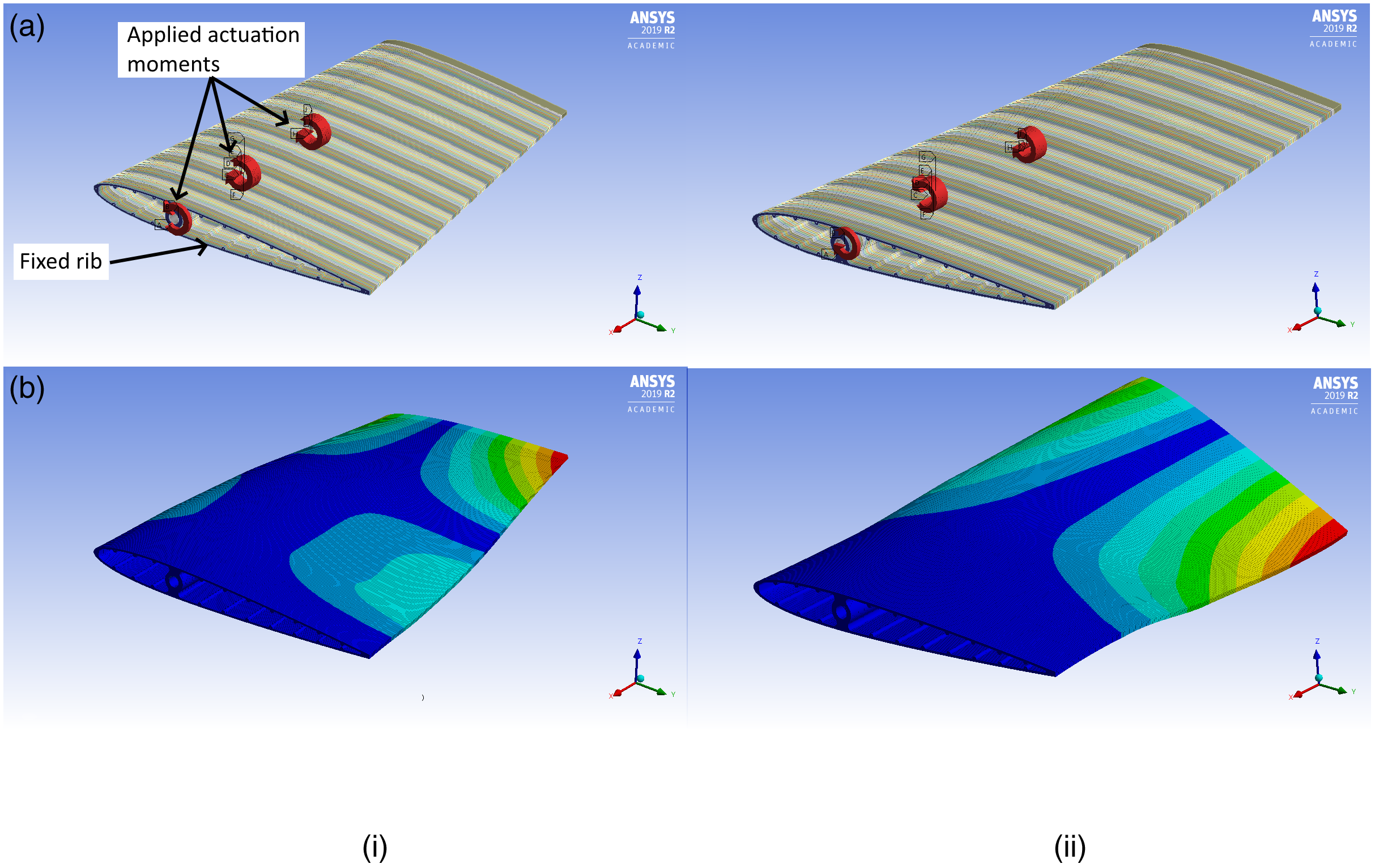
Figure 11. Two example FEA cases for the morphing section; (a) Configuration 1, (b) Configuration 3.
Table 3. Predicted and measured wing twist magnitudes for varying actuation configurations

3.5. Final morphing wing configuration and layout
These results provided the foundation for the construction of the morphing wing CAD design shown in Fig. 12. Overall, the design incorporates a morphing segment (0.215 < y/b < 0.5) with three independently actuated spanwise stations, together with a fixed, inboard section, for fuselage support. The three actuation stations are located at y/b = 0.298(AS1), y/b = 0.372(AS2) and at the wingtip (y/b = 0.5).

Figure 12. CAD model of morphing wing design (fixed section uncovered for clarity).
Four chordwise surface pressure stations designated PTS1-4 were also incorporated within the design to allow surface pressure measurement feedback. Two stations are coincident with AS1 and AS2 (PTS2 and PTS3 respectively) with PS4 positioned further outboard (y/b = 0.445). An additional inboard station (PTS1) was also installed at y/b = 0.128 (on the fixed portion) to provide a reference from which all other stations (PS2-4) could be compared (see Section 4). At each measurement position, a total of 14 individual pressure taps (7 top, 7 bottom) were embedded with an identical chordwise spatial distribution non-linearly bias towards the wing leading edge. This distribution is quantified in Table 4 (see also Fig. 16) and was used along with Equations (1) and (2) to resolve the sectional lift coefficient (Cl ’) at each spanwise station. Subsequent assessment of Cl ’ measurement uncertainty was better than ΔCl ’ = ±0.03 with all 56 pressure lines (per wing) gaining access to the fuselage via the fixed wing segment.
 \begin{align} {\left( {\boldsymbol{{C}}'_{\!\!\boldsymbol{{N}}}} \right)_{\boldsymbol{{n}}}}\; = {\boldsymbol\sum}_{\textbf{1}}^{\boldsymbol{{i}}} {\left( {{\boldsymbol{{C}}_{\boldsymbol{{p}},\boldsymbol{{l}}}} - {\boldsymbol{{C}}_{\boldsymbol{{p}},\boldsymbol{{u}}}}} \right)_{\boldsymbol{{n}}}}\boldsymbol{{d}}\!\left( {\boldsymbol{{x}}/\boldsymbol{{c}}} \right) \end{align}
 \begin{align} {\left( {\boldsymbol{{C}}'_{\!\!\boldsymbol{{l}}}} \right)_{\boldsymbol{{n}}}}\; = {\left( {\boldsymbol{{C}}'_{\!\!\boldsymbol{{N}}}} \right)_{\boldsymbol{{n}}}}\;\boldsymbol{{cos}}\!\left( \alpha\,\textbf{+}\,\gamma\right)({\boldsymbol{{c}}_{\boldsymbol{{n}}}}/\bar{\bar{\boldsymbol{{c}}}}) \end{align}
Table 4. Chordwise pressure tap locations used in the calculation of sectional lift coefficient

The means for independent spanwise twist control was provided by three concentric carbon-fibre torque tubes installed at the wing quarter-chord position. Each tube extended from the wing root to the corresponding actuation 5-rib combination (AS1-3) where they were all bonded in place. Machined aluminium ferrules ensured adequate separation between each tube giving near-frictionless operation. The fixed portion of the wing was used to provide primary structural support to the outermost torque tube with each tube connected to its own, independently controlled, actuation mechanism (see Section 3.7).
3.6. Morphing wing limits and capabilities
Prior to wind tunnel testing, a calibration of localised wing twist at each station (AS1-3) against applied moment was experimentally assessed. Table 3 includes these results with all angular measurements obtained using a Eflight AnglePro II digital incidence meter with a precision of Δγ = ±0.1°. Overall uncertainty in zero offset and hysteresis was Δγ = ±2°.
As shown in Table 3, these results show good agreement with those obtained from the FEA analysis. As predicted by the FEA, maximum twist occurs with all stations acting in unison to produce γtip = 22° (Configuration 2). The consequence of reversing direction at AS1 is shown to reduce the maximum achievable (γtip = 18° – Configuration 3) with further decreases if direction at both AS1 and AS2 is reversed (γtip = 10° – Configuration 4). Application at AS3 only (Configuration 0) is shown to be marginally less (γtip = 13.5°) than that used in the AVL analysis (γtip = 16° – see Section 3.2.1) likely resulting in actual roll performance being somewhat less than predicted. Further comparisons also highlight asymmetry based on applied moment direction (Configurations 3 and 6) as well as a general inter-dependence of any individual twist magnitude on the application status of the other two. Nevertheless, these experimental results again confirm the diversity of possible spanwise twist orientations available to the design with good agreement to those predicted by the FEA.
3.7. UAV platform re-design and modifications
A significant re-design of the baseline UAV internal structure was required to integrate each wing set. The primary modifications involved removal of the main fuselage brace and wing tube support to allow suitable access for the three-tier actuation system (AS1-3). These components, together with a carbon-fibre wing tube, provided primary resistance to wing-induced bending moment and needed a suitable replacement. Other elements to facilitate actuation, measurement and control feedback, also required integration with a final consideration being the need to incorporate the baseline wings within the same framework. The multi-tier actuation and control system is not required for the latter as pre-installed wing servos (at wing mid-span) are used for aileron control.
Internal design detail for each setup is shown in Figs. 13 and 14 (only starboard side components indicated). The basic philosophy behind the design was to split the original assembly along the aircraft centreline (port and starboard sections) while leaving front and rear frames, battery tray and frame braces unmodified. These provided a solid base for support while also allowing sufficient scope to add supplementary hardware and structural support to maintain adequate load transfer. This strategy also allowed positioning of linear accelerometer/gyro instrumentation at the aircraft centre of gravity for subsequent flight test analysis.

Figure 13. Internal design detail for the baseline wing setup (port side components and aircraft fuselage omitted for clarity).

Figure 14. Internal actuator design detail for the morphing wing configuration (selected components omitted for clarity).
Figure 13 shows underlying detail for the baseline wing configuration. Dummy servo assemblies are used in this instance as the primary wing load transfer mechanism onto the fuselage through a truncated carbon fibre wing tube (made from the original) and a custom wing-root support structure assembly bonded to the fuselage. Both bottom and top support plates (latter not shown for clarity) were affixed to each wing root (port and starboard) and used as a mount for the two dummy servo structures. Each truncated wing tube terminated at the inner-most edge of these structures leaving a central 5mm gap to position a ICM20649 6-axis accelerometer and gyro combination. This sensor measured linear acceleration and angular velocity about all three axes within a range of ±8 g and ±500 deg/s respectively (uncertainty ±0.03 g and ±1 deg/s).
Figure 14 provides detail of the morphing wing setup. Much of the assembly remains common, with wing root support structures and top/bottom support plates again utilised. Three separate and independently controllable servomechanism systems (AS1-3) are shown. The first two, AS1-2, used modified Hitec HS5087MH servos to act as linear actuators, with the third, AS3 (Savox SB-2290SG), left unaltered. The need for the former was required due to use of two separate aluminium control horns to actuate each corresponding torque tube (see Figs. 12 and 14 – AS1-2). AS3 was coupled directly to the innermost torque tube via a splined adaptor (see Fig. 12 – AS3).
Figure 15 provides a further outer layer of detail incorporating subsequent support systems and hardware common to both configurations. These include a carbon fibre top support plate, the MPS4264 Scanivalve (used for wing surface pressure data acquisition), a Raspberry Pi 4 microcomputer (1.5MHz Quad Core, 8GB RAM) as the primary computational resource and Pololu Jrk 21v3 motor controllers/Series 150 sub-miniature position transducers combinations to measure local wing twist (via connection to the aluminium control horns). In unison, all these systems provide the capability for real-time, independent measurement and closed-loop feedback control.

Figure 15. Basic acquisition and feedback/control instrumentation setup (port side components omitted for clarity).
Figure 16 shows the fully instrumented UAV prototype with the morphing wings installed. In addition to the MPS4264 Scanivalve, Raspberry Pi 4, Pololu Jrk 21v3 motor controllers, and Series 150 sub-miniature position transducers, a MATEK ASPD-7002 analog airspeed sensor was integrated to measure flight speed (via a pitot-static tube – not shown), a 4S Overlander lithium-polymer 3800mAh flight battery to provide common electromotive potential, a receiver for remote flight control, and an Adafruit Ultimate Global Positioning System (GPS) for the measurement of flight altitude and position.

Figure 16. Top view of modified UAV platform.
3.8. Electrical systems and integration
The overall power distribution and signal integration layout with the Raspberry Pi is shown in Fig. 17. A single, four-cell (14.8V), 3,800mAh lithium-polymer flight battery (1) provides sole electromotive potential for the entire UAV. This source supplies the Airboss 80 ESC (2), Xpwr T3910 brushless motor (3) and Xor 14x7 propeller (not indicated) combination for primary flight propulsion, a D36V28FS 5-volt Step-down voltage regulator (4) to power the Raspberry Pi (5), four Pololu Jrk 21v3 motor/position feedback controllers (6), and the MPS4264 Scanivalve (not indicated). A separate, integrated voltage source, embedded within the ESC is used to power the flight receiver (7), port and starboard aileron servos (8&9), as well as elevator and rudder servos (not shown – Hitec HS-5087MH); the latter using command signals directly from the flight receiver, and the former, from Raspberry Pi pins 13 and 12. Connections to pins 16, 20, and 21 log elevator, rudder and throttle demanded position with port and starboard command signals from the flight receiver first read by pins 7 and 1 before software manipulation and final transmission via pins 13 and 12, respectively.

Figure 17. UAV Instrumentation and system electrical layout.
All other instrumentation were powered from the internal Raspberry Pi 5V supply. These included an ADS1115 16-bit analog-to-digital converter (11) used to digitise analog airspeed (10), as well as the ICM20649 6-axis Accelerometer/Gyro (12) using the inbuilt Raspberry Pi I2C interface (100kHz clock frequency). Sample rates for both sensors were 1kHz with inbuilt low-pass sensor filters configurated at 200Hz. Pull-up resistors (5k ohms) connecting both the SDA and SCL lines and the 5V supply were employed to ensure reliable performance. The Raspberry Pi serial interface (baud rate = 9,600, sample rate = 10Hz) was also used to read all GPS data from an Adafruit Ultimate GPS (13) with a software-generated trigger (pin 26) adopted to allow synchronisation between the Raspberry Pi and the wind tunnel load cell (see Section 4). A hall-effect current sensor (14) and 4:1 voltage divider (15) connected to the ADS1115 provided motor input power available with rpm (16) measured via Pin 4 of the Raspberry Pi.
3.9. Feedback control setup
Basic functionality of the closed-loop feedback positioning system employed is depicted in Fig. 18. This system used a hybrid hardware/software-oriented PID control strategy using a user-specified sectional lift (Cl ’) distribution as the set point. Stations AS1-2 were hardware-controlled with the two Pololu 21v3 motor controllers per wing used to drive the two Hitec HS5087MH servos/control horn combinations (see Fig. 16). Position feedback at AS1-2 is provided by the two Series 150 sub-miniature position transducers with sensor output used as feedback to each Pololu Jrk 21v3. Control was inbuilt to each controller with each system requiring only initial tuning of PIDFootnote 6 constants (K P, K I, and K D) and a single PWM control signal from the Raspberry Pi.

Figure 18. Schematic of wing twist position closed-loop feedback control system.
This hardware-based configuration worked in unison with a similar, but separate, software-controlled strategy for AS3. For this system, calculated Cl ’ was again compared to a target, with corresponding PWM signal control again provided by the Raspberry Pi. A similar tuning process to that already described was also required.
3.10. Software development
The software developed to co-ordinate all UAV capabilities from the Raspberry Pi was written in Python 3.0 (linux-based version). This combination offered a fast, versatile and effective means for system and sensor integration while minimising weight and space requirements. Overall command and control was provided wirelessly via a laptop PC connected to a WiFi interface installed on the Raspberry Pi (mobile access point). A flowchart outlining basic operation is shown in Fig. 19.

Figure 19. Software flowchart highlighting signal integration and feedback control.
The first step executed by the code was to import all required software libraries to support sensor and system communication protocols, data manipulation and signal generation. System defaults and/or calibrated offsets and constants are thereafter defined before initialising all embedded sensors and systems for data transfer. The output data file is also created and configured at this stage with designated column headers included. Reference atmospheric data (temperature, pressure) required for subsequent calculations (density, dynamic pressure, etc.) are also thereafter provided along with sensor zero offset corrections.
Further program constants and defaults follow in the next step including defining UAV geometric configuration and setup constraints, Raspberry Pi pin number designations and output state, PWM signal defaults and limits, position feedback settings, as well as retrieving a timestamp reference. Subsequent entry into the main program loop thereafter initiates a trigger signal allowing synchronisation with load cell measurements along with calculation of real-time flow speed from dynamic pressure (required for C l ’). Data release commanded to the inbuilt FTP server of the Scanivalve provided the raw information for this operation, with current wing twist positions (AS1-3) also measured. Comparisons between target and measured sectional lift spanwise distributions is then made through the PID controllers with amendments to each PWM signal width commanded until an acceptable match was achieved (maximum 5% difference set); further signal modifications ceasing thereafter. This loop persisted until either an aerodynamic change occurs, or a commanded program exit is given; the latter action ceasing all computations. The maximum update rate is 30Hz.
4. Experimental setup and apparatus
4.1. Wind tunnel
The model was tested in a closed-circuit wind tunnel with a maximum flow velocity of 60 m/s and a closed-test section measuring 1.68 × 1.22 m. Maximum model blockage based on projected frontal area at maximum angle-of-attack (α = 15°) and zero yaw was 5.3% with the installed wing span extending up to 79% of the tunnel width. No corrections for these influences were applied to the results given the comparative nature of the study. The turbulence intensity at model station is rated at lower than 0.2% with operating flow speeds limited to between 18 and 25m/s depending on the test undertaken. These conditions gave a Reynolds number range, based on mean aerodynamic chord, of 3.72 × 10⁵ < Ren < 4.68 × 10⁵.
The model was mounted on an aerodynamically streamlined support strut affixed to an aluminium floor insert installed within the tunnel floor. A six-axis load cell was positioned between the model support strut and the floor insert to allow all forces and moments acting on the model to be measured. An angle-of-attack adjustment mechanism (−1.8° < α < 15°, Δα $\thickapprox$
2.5°) also allowed assessment of this influence on aerodynamic performance. To ensure minimal aerodynamic disturbance, a two-piece, flat plate wooden cover, sealed the resulting open space between the support strut and floor insert leaving a nominal 5mm gap to allow unhindered support strut deflection under aerodynamic loading. This also minimised external air ingress into the tunnel. Figure 20 shows both model configurations installed in the wind tunnel prior to testing.
$\thickapprox$
2.5°) also allowed assessment of this influence on aerodynamic performance. To ensure minimal aerodynamic disturbance, a two-piece, flat plate wooden cover, sealed the resulting open space between the support strut and floor insert leaving a nominal 5mm gap to allow unhindered support strut deflection under aerodynamic loading. This also minimised external air ingress into the tunnel. Figure 20 shows both model configurations installed in the wind tunnel prior to testing.

Figure 20. Wind tunnel installations of the model configurations: (a) Baseline, (b) Morphing.
The angle of wing twist at each station (AS1-3) prior to testing was calibrated in situ using the Eflight AnglePro II digital incidence meter. This process involved initially measuring the angle of incidence and either disconnecting the corresponding leadscrew actuator (AS1-2) for adjustment or modifying input signal magnitude directly via the software. After calibration, maximum deviation between any station, on either wing, was found to be less than Δγ = ±2°.
4.2. Data acquisition and equipment setup
An AMTI MC3A-500 six-axis force and moment balance was used during wind tunnel testing. The maximum lift, drag and side force capabilities of the cell were ±2kN, ±1kN, and ±1kN respectively, with the maximum range for pitching, rolling and yawing moments being ±56Nm, ±56Nm and ±28Nm respectively. During initial testing, individually optimised measurement ranges were set for all six-axes using a DigiAmp DSA-6 amplifier to minimise data uncertainty. After calibration, maximum deviations for any axis was found to be less than ±2.5% with 95% confidence.
All aerodynamic force and moments were acquired using a CompactRIO 9025 running a 16-bit NI9025 Analog Input module. This system used custom-programmed Labview FPGA control architecture linked to an external laptop to coordinate the process. The sampling rate was 10kHz with internal low-pass Butterworth filters within the DigiAmp configured at 1kHz to satisfy the Nyquist anti-aliasing criterion. The software trigger from the Raspberry Pi was connected to an additional channel to provide synchronisation between both systems. All time-averaged data were sampled for a minimum period of 20 s with tests involving wing transitioning from one state to another extending to up to 120 s. Before and after every test, a zero, wind-off, data point was taken. This allowed compensation of any thermal drift measurement zeros, the identification of superfluous, non-aerodynamic, frequency components, as well as inclusion of reference data required by the control software. Additional tests were also performed without the model installed to correct for support tare.
The Matek ASPD-7002 airspeed sensor/pitot static tube combination was calibrated in situ against a Dantec© precision flow unit with rated accuracy better than ±0.5m/s. This procedure involved positioning the flow unit discharge orifice within 5mm of the pitot-static tube leading edge and progressively increasing speed up to 40 m/s (steps of 5 m/s) before being reduced back to zero. This methodology was adopted to assess hysteresis and repeatability with overall calibration offset and gain constants determined as the average of three separate calibration events. Final accuracy was assessed at better than ±1m/s to 95% confidence.
5. Results and discussion
5.1. Baseline comparisons
Baseline aerodynamic performance comparisons for the two model configurations tested are provided in Fig. 21. Overall, the drag polars show good agreement over the entire angle-of-attack range considered with some variation at higher lift coefficients near stall (12.2° < α < 15°). The morphing wing variant was found to produce the lowest minimum drag coefficient (C
D = 0.0392) with the baseline marginally higher (C
D = 0.0446); each observed at α = 0.6°. For the latter, the influence of the exposed aileron wing servos and control horns as well as control surface hinge junctions likely contributed to this difference. Maximum lift coefficient is in general agreement for both (C
Lmax $\thickapprox$
1 at α = 12°) with the maximum lift-to-drag ratio observed at (C
L/C
D)max = 9.18, and (C
L/C
D)max = 10.66 respectively; both at α = 7.1°. These results indicate a 16% increase in aerodynamic efficiency with use of the ATC concept reaffirming results from previous exploratory work [Reference Kaygan and Gatto21]. Comparing results obtained from both the CFD and AVL analysis (Fig. 5) also show general agreement.
$\thickapprox$
1 at α = 12°) with the maximum lift-to-drag ratio observed at (C
L/C
D)max = 9.18, and (C
L/C
D)max = 10.66 respectively; both at α = 7.1°. These results indicate a 16% increase in aerodynamic efficiency with use of the ATC concept reaffirming results from previous exploratory work [Reference Kaygan and Gatto21]. Comparing results obtained from both the CFD and AVL analysis (Fig. 5) also show general agreement.

Figure 21. Drag polar comparison for the two model variants; Ren = 3.72x10⁵.
Further insight into overall wing behaviour is presented in Fig. 22. These results show spanwise C
l
’ variation (C
l0-3’) from stations PTS1-4 (see Fig. 12) at different α. As would be expected, C
l
’ magnitudes progressively increase with α maintaining a near common profile up to α $\thickapprox$
10°. Beyond α = 12.2° however, little further change at innermost stations (C
l0-2’) is seen suggesting aerodynamic behaviour typical near stall. Further increase to α = 15° also shows a subtle inboard unloading at C
l0
’ and C
l1
’ typical of the same cause. Loading at the tip however remains essentially unchanged, indicating the basic wing configuration has a preference to stall at the wing root first, prior to the tip, as would be most desired to maintain roll control.
$\thickapprox$
10°. Beyond α = 12.2° however, little further change at innermost stations (C
l0-2’) is seen suggesting aerodynamic behaviour typical near stall. Further increase to α = 15° also shows a subtle inboard unloading at C
l0
’ and C
l1
’ typical of the same cause. Loading at the tip however remains essentially unchanged, indicating the basic wing configuration has a preference to stall at the wing root first, prior to the tip, as would be most desired to maintain roll control.

Figure 22. Sectional lift distribution profiles with change in α for the morphing configuration.
Figure 23 provides these results normalised against C l0’ for assessment against an elliptic profile (minimum induced drag) [Reference Phillips, Fugal and Spall17, Reference Phillips20, Reference Lane, Marshall and Mcdonald27]. As shown, the C l’ distribution in most cases (with the possible exception of α = −1.8) varies from this ideal (outboard stations more loaded) indicating scope does exist for optimisation (through wing twist adjustment) at multiple flight orientations (i.e. non cruise conditions). This will be demonstrated in following sections.

Figure 23. Measured normalised sectional lift distributions compared to the elliptic profile.
5.2. Adaptability limits
Prior to demonstrating this capability however, wind tunnel tests to establish maximum achievable C L and C D ranges were performed. For these tests, each actuator station was commanded to maximum positive twist magnitude (see Table 3) with subsequent separate tests, considering negative thereafter.
Figures 24 and 25 show the range of achievable C L, C D, ΔC L and ΔC D respectively. From Fig. 24, nominal C L and C D (γ = 0 at AS1-3) is shown to lie within an upper and lower bound with available range tightening notably for C L at high α (approaching stall − α > 10°). The reverse is evident for C D. For the former, these results show that near maximum aerodynamic loading, additional benefits from ATC use are more limited. At lower α however, C L is shown to have the capability for significant change; that being near equal (constant ΔC L) in either direction from γ = 0. This is maximum at ΔC L = 0.27 for α = 3° (Fig. 25).

Figure 24. Maximum C L and C D limits achievable for the morphing wing; Ren = 3.72x10⁵.

Figure 25. Achievable ΔC L and ΔC D for the morphing wing; Ren = 3.72x10⁵.
Conversely, Fig. 24 shows most C
D variability is enabled at higher α and more limited at low α. This is a result of the wing already being in a low drag state for the latter with either positive or negative γ change (from γ = 0) producing a net increase. The no twist, low drag condition (γ = 0), therefore lies outside the measured upper and lower bound as C
D is lower in both cases. Only at α $\thickapprox$
3° does C
D for γ = 0 enter the bounded range remaining within thereafter. A bias towards the lower bound is also observed, in opposition to that observed for C
L, suggesting limited additional gains exist through reducing C
D within this α range. Figure 25 quantifies this finding for α ≤ 4.9° with ΔC
D < 0.04 much lower than ΔC
D
$\thickapprox$
3° does C
D for γ = 0 enter the bounded range remaining within thereafter. A bias towards the lower bound is also observed, in opposition to that observed for C
L, suggesting limited additional gains exist through reducing C
D within this α range. Figure 25 quantifies this finding for α ≤ 4.9° with ΔC
D < 0.04 much lower than ΔC
D $ > $
0.09 at α ≥ 10°. Most benefit therefore, in terms of reducing C
D, will exist at the highest α (near stall). Considered in unison with C
L, these results confer significant enhancements in C
L/C
D with ATC use, particularly above and below (C
L/C
D)max. This can be realised most effectively by enacting a positive γ change (increasing C
L more than the relative increase in C
D) at low α, thereby increasing C
L/C
D, and using negative γ change (to reduce C
D more than the relative reduction in C
L) at high α, again increasing C
L/C
D. This capability is demonstrated in the next section.
$ > $
0.09 at α ≥ 10°. Most benefit therefore, in terms of reducing C
D, will exist at the highest α (near stall). Considered in unison with C
L, these results confer significant enhancements in C
L/C
D with ATC use, particularly above and below (C
L/C
D)max. This can be realised most effectively by enacting a positive γ change (increasing C
L more than the relative increase in C
D) at low α, thereby increasing C
L/C
D, and using negative γ change (to reduce C
D more than the relative reduction in C
L) at high α, again increasing C
L/C
D. This capability is demonstrated in the next section.
To further quantify the nature of the effects of γ on C
l’, Figs. 26 and 27 provide the corresponding upper and lower bound for C
l’ together with ΔC
l’. At the most inboard measurement station (C
l0’) at high α (α $\thickapprox$
10°), little impact on C
l’ occurs with changing γ confirming the trend identified earlier in Fig. 22. The influence of γ change is shown to increase progressively out to the wing tip however, where ΔC
l’ is maximum, indicating, as suspected earlier, relative insensitivity of C
L to γ at highest aerodynamic loading. Conversely, at lower α, the ability to modify C
l’ changes markedly at all spanwise positions, particularly those innermost (C
l0-2’), with near-constant ΔC
l’ capability observed below α = 4.9°. Maximum limits are quantified in Fig. 27 with ΔC
l3’
$\thickapprox$
10°), little impact on C
l’ occurs with changing γ confirming the trend identified earlier in Fig. 22. The influence of γ change is shown to increase progressively out to the wing tip however, where ΔC
l’ is maximum, indicating, as suspected earlier, relative insensitivity of C
L to γ at highest aerodynamic loading. Conversely, at lower α, the ability to modify C
l’ changes markedly at all spanwise positions, particularly those innermost (C
l0-2’), with near-constant ΔC
l’ capability observed below α = 4.9°. Maximum limits are quantified in Fig. 27 with ΔC
l3’ $\thickapprox$
0.2 (independent of
$\thickapprox$
0.2 (independent of $\alpha$
), ΔC
l1-2’
$\alpha$
), ΔC
l1-2’ $\thickapprox$
0.25, and ΔC
l0’
$\thickapprox$
0.25, and ΔC
l0’ $\thickapprox$
0.16), respectively. Figure 27 also highlights a rapid decrease in ΔC
l’ for α ≥ 7° at C
l0-2’ as stall is approached, however, as the ability to tailor γ (in this case reduce) would offer scope for mitigation. Such characteristics may also provide benefits for tailoring C
L and C
D needs based on take-off and landing requirements [Reference Scherer13, Reference Martin, Kudva, Austin, Jardine and Scherer28, Reference Falca, Gomes and Suleman29] as well as the reduction of stall speed [Reference Falca, Gomes and Suleman29].
$\thickapprox$
0.16), respectively. Figure 27 also highlights a rapid decrease in ΔC
l’ for α ≥ 7° at C
l0-2’ as stall is approached, however, as the ability to tailor γ (in this case reduce) would offer scope for mitigation. Such characteristics may also provide benefits for tailoring C
L and C
D needs based on take-off and landing requirements [Reference Scherer13, Reference Martin, Kudva, Austin, Jardine and Scherer28, Reference Falca, Gomes and Suleman29] as well as the reduction of stall speed [Reference Falca, Gomes and Suleman29].

Figure 26. Measured C l’ limits at selected α for the morphing wing at C l0-3’; Ren = 3.72 × 10⁵.

Figure 27. Achievable ΔC l’ for the morphing wing at C l0-3’; Ren = 3.72 × 10⁵.
5.3. Real-time flight optimisation
Having assessed nominal aerodynamic performance metrics as well as overall limits and capabilities, focus hereafter centres on the ability to provide real-time enhanced flight efficiency. To demonstrate this capability, tests were performed whereby the morphing wing was commanded to transition from neutral to maximum wing twist, then back to neutral, and then fully negative. This strategy would take advantage of the simultaneous force and moment measurement capability of the experimental setup to quantify how these parameters can be modified real-time to improve flight efficiency. The maximum duration for these tests was 120 s and are considered quasi-steady in nature.
Example cases taken at α = 2.2° and α = 12.2° are shown in Figs. 28 and 29; the former applying positive γ, and the latter, negative. Calculated C
L/C
D and a synchronising trigger signal (between model and load cell) are also shown. In each case, full transition occurs after approximately 20 s. From Fig. 28, this action increases C
L from C
L $\thickapprox$
0.26 to C
L
$\thickapprox$
0.26 to C
L $\thickapprox$
0.5 representing a 92% increase. Drag coefficient also increases during the same period from C
D
$\thickapprox$
0.5 representing a 92% increase. Drag coefficient also increases during the same period from C
D $\thickapprox$
0.041 to C
D
$\thickapprox$
0.041 to C
D $\thickapprox$
0.057 (39% increase), however C
L/C
D improves from C
L/C
D
$\thickapprox$
0.057 (39% increase), however C
L/C
D improves from C
L/C
D $\thickapprox$
7 to C
L/C
D
$\thickapprox$
7 to C
L/C
D $\thickapprox$
9.6 (37% increase). Conversely, Fig. 29 (α = 12.2°) shows C
D reducing to C
D
$\thickapprox$
9.6 (37% increase). Conversely, Fig. 29 (α = 12.2°) shows C
D reducing to C
D $\thickapprox$
0.098 from C
D
$\thickapprox$
0.098 from C
D $\thickapprox$
0.21 (−53%) with C
L reducing from C
L
$\thickapprox$
0.21 (−53%) with C
L reducing from C
L $\thickapprox$
1 to C
L
$\thickapprox$
1 to C
L $\thickapprox$
0.88 (−12%). This modification again improves C
L/C
D (88%). Figure 30 shows the modified wing C
l’ distribution in each case, with the loading at the tip increasing markedly for α = 2.2° and reducing at α = 12.2°.
$\thickapprox$
0.88 (−12%). This modification again improves C
L/C
D (88%). Figure 30 shows the modified wing C
l’ distribution in each case, with the loading at the tip increasing markedly for α = 2.2° and reducing at α = 12.2°.

Figure 28. Real-time C L/C D enhancement from the morphing wing at α = 2.2°; Ren = 3.72 × 10⁵.

Figure 29. Real-time C L/C D enhancement from the morphing wing at α = 12.2°; Ren = 3.72 × 10⁵.

Figure 30. Results for C l’ during real-time transition at Ren = 3.72 × 10⁵; α = 2.2°(dashed), α = 12.2°(solid).
Figure 31 provides a full assessment of this capability by quantifying maximum measured improvement in flight efficiency over the full α range. Achievable benefit is shown throughout, albeit much more subtle near (C L/C D)max (6.4% at α = 7°). Again, this was expected as the platform is near optimum aerodynamic performance at this α making additional gains more difficult. Most benefit is shown either side of this location, with the maximum observed at lowest α. Overall 6.4% < ΔC L/C D < 72% was obtained within 2.2° < α < 15° demonstrating an ability to both increase achievable C L/C D (at any fixed α) as well as expand the α range for fixed C L/C D (note: below this range the % gains are much larger). Given many critical performance metrics use C L/C D (range, endurance, etc.), these findings highlight the possibility to deliver significant improvements in real-time flight adaptability.

Figure 31. Overall improvement in C L/C D using the morphing wing; Ren = 3.72 × 10⁵.
5.4. Closed-loop feedback control
Closed-loop feedback control was the next capability investigated. This functionally was incorporated within the hardware and software control architecture to automatically adjust, and maintain, any specified C l’ distribution. Tests to demonstrate this ability were performed with a target elliptical lift distribution [Reference Phillips20].
Real-time evolution of C
l0-3’ from loop initiation (t = 0) at α = 10° is shown in Fig. 32. For t < 7 s, the highly unsteady nature of the flowfield, typical to conditions approaching aerodynamic stall, can be clearly identified. Quantitative assessment within this region indicates C
Lrms $\thickapprox$
0.017 and C
Drms
$\thickapprox$
0.017 and C
Drms $\thickapprox$
0.006, respectively, with the same metrics after actuation (t > 7) showing a significant reduction as aerodynamic unloading of the wing tip occurs (C
Lrms
$\thickapprox$
0.006, respectively, with the same metrics after actuation (t > 7) showing a significant reduction as aerodynamic unloading of the wing tip occurs (C
Lrms $\thickapprox$
0.002, C
Drms
$\thickapprox$
0.002, C
Drms $\thickapprox$
0.0005). These results suggest benefits may also exist for stall mitigation (a reduction in model unsteadiness was also observed visually – see [22]). During the subsequent transition however, C
l1-3’ are all shown to change magnitude (C
l0’ remaining constant) to meet the target C
l’ distribution. Results reach a steady-state condition by t
$\thickapprox$
0.0005). These results suggest benefits may also exist for stall mitigation (a reduction in model unsteadiness was also observed visually – see [22]). During the subsequent transition however, C
l1-3’ are all shown to change magnitude (C
l0’ remaining constant) to meet the target C
l’ distribution. Results reach a steady-state condition by t $\thickapprox$
30 s with excellent agreement achieved between final and target C
l’ (see Fig. 33). Multimedia demonstrating this test is available to view at [22].
$\thickapprox$
30 s with excellent agreement achieved between final and target C
l’ (see Fig. 33). Multimedia demonstrating this test is available to view at [22].

Figure 32. Evolution of the C l’ distribution to achieve an elliptical lift distribution; α = 10°, Ren = 4.68 × 10⁵.

Figure 33. Normalised C l’ distribution demonstrating closed-loop feedback control for minimum drag at α = 10°; Ren = 4.68 × 10⁵.
5.5. Manoeuvre load alleviation
A further capability is the potential for Manoeuvre Load Alleviation [Reference Miller5, Reference Vasista, Tong and Wong12]. This is a condition whereby wing loading is increased inboard and relaxed outboard during flight manoeuvring to reduce generated wing root bending moment. The same functionality described in Section 5.4, but with an appropriately set target C l’ distribution (see Fig. 35), was used.
Figures 34 and 35 provide the real-time and normalised C
l’ results at α = 4.9° from such a test. Again, C
l’ magnitudes after initiation (t = 0) are seen to progressively change during transition, with an increased inboard loading required by MLA shown by C
l1’ increasing beyond C
l0’ ( $\thickapprox$
10%) at t = 35 s. This change is also highlighted in Fig. 35. Aerodynamic loading at both C
l0’ and C
l2’ remains relatively unchanged however, with C
l3’ reducing significantly (ΔC
l3’
$\thickapprox$
10%) at t = 35 s. This change is also highlighted in Fig. 35. Aerodynamic loading at both C
l0’ and C
l2’ remains relatively unchanged however, with C
l3’ reducing significantly (ΔC
l3’ $\thickapprox$
0.06 to C
l3’/Cl0’
$\thickapprox$
0.06 to C
l3’/Cl0’ $\thickapprox$
0.46) as unloading of the wing tip compensates for the increase at C
l1’ to maintain near-constant C
L.
$\thickapprox$
0.46) as unloading of the wing tip compensates for the increase at C
l1’ to maintain near-constant C
L.

Figure 34. Real-time evolution of the morphing wing C l’ distribution to achieve MLA at α = 4.9°; Ren = 3.74 × 10⁵.

Figure 35. Normalised wing C l’ distribution demonstrating MLA at α = 4.9°; Ren = 3.74 × 10⁵.
5.6. Roll control effectiveness and efficiency
The final tests conducted involved comparing roll control power (C lγ, C lξ) and roll control power per unit ΔC D(C lγ/ΔC D, C lξ/ΔC D). These metrics provide comparable indications of how effectively (C lγ, C lξ) and efficiency (C lγ/ΔC D, C lξ/ΔC D) each wing provides roll performance. For these tests, maximum control deflections were commanded (see Tables 1, 2 and 3) for each wing configuration. For this comparison, note should be made however that near full span ailerons (90% - see Section 3.1) are used for the baseline wing; this being an atypical configuration not representative of most aircraft configurations (10%–30% is more typical [Reference Vos, de Breuker, Barrett and Tiso14]). This would be expected to underpredict comparative ability of the morphing wing. Also of note is that this test does not include comparative assessment of intermediate morphing wing (and baseline aileron) configurations which may prove more beneficial [Reference Pecora, Amoroso and Lecce3, Reference Abdulrahim, Garcia, Ivey and Lind9]. Nevertheless, the comparison was still considered valuable.
Figure 36 provides these results with both wing configurations shown to produce comparable roll control power. At C
lγmax $\thickapprox$
0.147 (α = 7°) and C
lξmax
$\thickapprox$
0.147 (α = 7°) and C
lξmax $\thickapprox$
0.255 (α = 10°) these values approximate that of typical aircraft (C
lξ
$\thickapprox$
0.255 (α = 10°) these values approximate that of typical aircraft (C
lξ $\thickapprox$
0.3 – [Reference Gilyard30]). Aileron control power (C
lξ) under these conditions is shown to be higher at all α compared to that available from the morphing wing, with this disparity increasing markedly near stall (α ≥ 10°). At these α, morphing control power is shown to reduce significantly matching the trend already observed in Figs. 24, 25, 26 and 27. It should also be noted that the role of structural deformation at these highly loaded conditions could not be accurately assessed (given the difficulty of measurement within an operating wind tunnel) and most likely would have some impact(increase) in wing twist measurement uncertainty [Reference Scherer13, Reference Stanford, Abdulrahim, Lind and Ifju25]. Noting this however, during testing very little noticeable deformation was visually observed.
$\thickapprox$
0.3 – [Reference Gilyard30]). Aileron control power (C
lξ) under these conditions is shown to be higher at all α compared to that available from the morphing wing, with this disparity increasing markedly near stall (α ≥ 10°). At these α, morphing control power is shown to reduce significantly matching the trend already observed in Figs. 24, 25, 26 and 27. It should also be noted that the role of structural deformation at these highly loaded conditions could not be accurately assessed (given the difficulty of measurement within an operating wind tunnel) and most likely would have some impact(increase) in wing twist measurement uncertainty [Reference Scherer13, Reference Stanford, Abdulrahim, Lind and Ifju25]. Noting this however, during testing very little noticeable deformation was visually observed.

Figure 36. Roll control power(solid line) and roll control power per unit change in drag coefficient(dashed line); Ren = 3.72x10⁵.
A comparison of roll control power efficiency (C
lγ,ξ/ΔC
D) is also provided in Fig. 36. These results show the morphing wing to be much more effective at efficiently producing roll control power relative to aileron use. For the latter, this metric is shown to remain relatively constant at C
lξ/ΔC
D $\thickapprox$
3 over the complete α range tested. Conversely, using morphing wing twist provides a capability up to C
lγ/ΔC
D = 35 with a near maximum 12:1 advantage (α
$\thickapprox$
3 over the complete α range tested. Conversely, using morphing wing twist provides a capability up to C
lγ/ΔC
D = 35 with a near maximum 12:1 advantage (α $\thickapprox$
7°).
$\thickapprox$
7°).
6. Conclusion
This paper describes the design, development, integration and testing of a morphing wing warping technology embedded with closed-loop feedback control capabilities onto a generic UAV platform to enhance performance, efficiency and control capabilities. Detailed descriptions of the design, control software architecture, electrical system layout, as well as assessments of realisable limits and capabilities are included together with results from a wind tunnel test program.
Two sets of wings with identical dimensions are compared; one utilising the morphing concept, and the other, a baseline configuration with embedded ailerons. The morphing wing utilised a segmented assembly of multiple, small thickness, rigid-rib sections, positioned directly adjacent, that possessed the ability for relative rotation over the affected span allowing localised wing twist variations. Subsequent wind tunnel testing showed the wing-warping technology to be superior in almost every comparative flight performance, efficiency and control metric investigated with the most significant realisable benefits being;
-
No increase in minimum drag.
-
Ability to modify C L and C D by up to a ΔC L = 0.27 and ΔC D = 0.12 respectively based on need without baseline angle-of-attack change.
-
Improved (C L/C D)max by 6.4%.
-
Improvement in C L/C D by 72% at α = 12.2°.
-
Capability for real-time wing load optimisation, closed-loop feedback control, and manoeuvre load alleviation.
-
Increase in roll control power efficiency by up to 12:1 compared to aileron use.
Overall, these findings highlight the possibility that the technology developed can provide a path to a functional, realistic and deployable step change in achievable aerial performance. Additional potential benefits yet to be fully explored and quantified, but warranting further investigation, could also include the reduction in radar cross-section signature, supermanoeuvrability, enhanced flight stability and gust load alleviation, as well as active flutter and structural vibration suppression. Ongoing work also involves application of the technology to rotary-wing platforms along with the development of a ‘water-tight’ variant using lightweight and flexible inter-rib materials to provide the required twist compliance.
Acknowledgments
I am deeply indebted to Robert Sayers and Matthew Stowell of DSTL for allowing this project to proceed in the midst of a global pandemic. Without their patience, understanding and financial support, none of this work would have been possible. I would also like to express my deepest gratitude to Jake Rigby of BMT for supporting this project from its inception. His advice has been invaluable throughout the entire process. Will Graham and Holger Babinsky of Cambridge University also deserve my sincere thanks for finding a way to allow the wind tunnel testing to proceed.
Funding
This work was financially supported by the Defence Science and Technology Laboratory (DSTL) for the UK Ministry of Defence(MoD) under Contract No. DSTLX1000146053 ‘Morphing Unmanned Aerial Vehicles (MORPHUAV): Realising Future Flight Capabilities’.


 Open access